Hoppa till huvudinnehåll

Hur markerar jag aktiv cell eller markering i Excel?

Om du har ett stort kalkylblad kanske det är svårt för dig att snabbt ta reda på den aktiva cellen eller det aktiva urvalet. Men om den aktiva cellen / sektionen har en enastående färg, kommer det inte att vara ett problem att ta reda på det. I den här artikeln kommer jag att prata om hur man automatiskt markerar den aktiva cellen eller det valda cellområdet i Excel.

Markera aktiv cell eller markering med VBA-kod


pil blå höger bubbla Markera aktiv cell eller markering med VBA-kod

Följande VBA-kod kan hjälpa dig att markera den aktiva cellen eller ett urval dynamiskt, gör så här:

1. Håll ner ALT + F11 nycklar för att öppna Microsoft Visual Basic for Applications-fönstret.

2. Sedan Välj Denna arbetsbok från vänster Project Explorerdubbelklicka på den för att öppna Modulerna, och kopiera och klistra sedan in följande VBA-kod i den tomma modulen:

VBA-kod: Markera aktiv cell eller markering

Sub Workbook_SheetSelectionChange(ByVal Sh As Object, ByVal Target As Excel.Range)
'Update 20140923
Static xLastRng As Range
On Error Resume Next
Target.Interior.ColorIndex = 6
xLastRng.Interior.ColorIndex = xlColorIndexNone
Set xLastRng = Target
End Sub

doc-highlight-active-cell-1

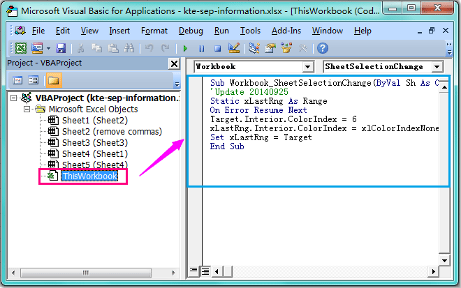
3. Spara och stäng sedan den här koden och gå tillbaka till kalkylbladet, när du väljer en cell eller ett val markeras de markerade cellerna och den flyttas dynamiskt när de markerade cellerna ändras.

Anmärkningar:

1. Om du inte hittar Project Explorer-rutan i fönstret kan du klicka utsikt > Project Explorer i Microsoft Visual Basic for Applications-fönstret för att öppna den.

2. I ovanstående kod kan du ändra .ColorIndex = 6 färg till annan färg du gillar.

3. Denna VBA-kod kan tillämpas på alla kalkylblad i arbetsboken.

4. Om det finns några färgade celler i kalkylbladet försvinner färgen när du klickar på cellen och sedan flyttar till en annan cell.


Relaterad artikel:

Hur markerar jag rad och kolumn för aktiv cell automatiskt i Excel?

Bästa kontorsproduktivitetsverktyg

🤖 Kutools AI Aide: Revolutionera dataanalys baserat på: Intelligent utförande   |  Generera kod  |  Skapa anpassade formler  |  Analysera data och generera diagram  |  Anropa Kutools funktioner.
Populära funktioner: Hitta, markera eller identifiera dubbletter   |  Ta bort tomma rader   |  Kombinera kolumner eller celler utan att förlora data   |   Rund utan formel ...
Superuppslag: Flera kriterier VLookup    VLookup med flera värden  |   VSök över flera ark   |   Fuzzy Lookup ....
Avancerad rullgardinslista: Skapa snabbt en rullgardinslista   |  Beroende rullgardinslista   |  Flervals-rullgardinslista ....
Kolumnhanterare: Lägg till ett specifikt antal kolumner  |  Flytta kolumner  |  Växla synlighetsstatus för dolda kolumner  |  Jämför intervall och kolumner ...
Utvalda funktioner: Rutnätsfokus   |  Designvy   |   Stor formelbar    Arbetsbok & Bladhanterare   |  Resursbibliotek (Automatisk text)   |  Datumväljare   |  Kombinera arbetsblad   |  Kryptera/Dekryptera celler    Skicka e-postmeddelanden efter lista   |  Superfilter   |   Specialfilter (filtrera fet/kursiv/genomstruken...) ...
Topp 15 verktygssatser12 text verktyg (lägga till text, Ta bort tecken, ...)   |   50+ Diagram Typer (Gantt Chart, ...)   |   40+ Praktiskt Formler (Beräkna ålder baserat på födelsedag, ...)   |   19 Införande verktyg (Infoga QR-kod, Infoga bild från sökväg, ...)   |   12 Konvertering verktyg (Siffror till ord, Valutaväxling, ...)   |   7 Slå ihop och dela verktyg (Avancerade kombinera rader, Dela celler, ...)   |   ... och mer

Uppgradera dina Excel-färdigheter med Kutools för Excel och upplev effektivitet som aldrig förr. Kutools för Excel erbjuder över 300 avancerade funktioner för att öka produktiviteten och spara tid.  Klicka här för att få den funktion du behöver mest...

Beskrivning


Fliken Office ger ett flikgränssnitt till Office och gör ditt arbete mycket enklare

  • Aktivera flikredigering och läsning i Word, Excel, PowerPoint, Publisher, Access, Visio och Project.
  • Öppna och skapa flera dokument i nya flikar i samma fönster, snarare än i nya fönster.
  • Ökar din produktivitet med 50 % och minskar hundratals musklick för dig varje dag!
Comments (16)
No ratings yet. Be the first to rate!
This comment was minimized by the moderator on the site
I had the same problem, read the whole page and comments. While thinking to apply it or not, I was just randomly clicking on number and letters to select the whole column and rows. Then suddenly highlight of selected cell feature came back :)
This comment was minimized by the moderator on the site
Hello, if someone can help me... I pick up this code in internet (apologies to the owner). It does almost what i need but this code select the entirerow. What i need is a change that alow to select just the first two cells of the row of the activecells. When i click in the cell, i need that the cell of the column "$I16" and "$J16" (16 is the first line of my table) of that row became interior color (=9359529). The code is this: 
Dim lTarget As Range

Private Sub Worksheet_SelectionChange(ByVal Target As Range)

If Target.Row >= 16 Then

If Not lTarget Is Nothing Then

lTarget.EntireRow.Interior.ColorIndex = 0
End If

Target.EntireRow.Interior.Color = 9359529

Set lTarget = Target
End If
End Sub

Can you help me? I had try to change this code but the only thing i can as the select the interior color of the cell target and not the column "$I" and "$J" in that specific row.Thank you for your help.
Luis Lopes
This comment was minimized by the moderator on the site
I know that you proposed a solution but the solution comes with another problem as you described below: "The only problem with having this code active is that you can no longer change the active cell color as it changes back to what it was before you clicked it. I suggest that if you need to change the highlight colors on the sheet, do so with macros disabled or change the sub name for a second so it doesn't trigger when you are clicking on cells". This is not an acceptable alternative for me. I need to be able to change the colors in the cells when the macro is active. Do you have a solution for this this problem. If you come up with a solution for this problem please republish your corrected macro the new macro in full (rather than proposing patches to your original macro because I am technically challenged as far as macro are concerned).
This comment was minimized by the moderator on the site
I tried your macro by copying and pasting it into my Excel file. I did change one thing in the macro though. I changed the color index from 6 to 24 (to a color different than the colors I am currently using in my macro). It worked very nicely and I liked it a lot but then started causing a problem for me. I have a lot of cells filled with with colors in my Excel. The macro started removing the color fill from every cell touched. I don't know how to stop the macro's this odd behavior. I did not have any choice but to remove the macro from my file. I still like to use this macro if someone can help me to fix it.
This comment was minimized by the moderator on the site
That was super helpful, thank you.
This comment was minimized by the moderator on the site
Anyway you can do the left adjacent cell to highlight instead of active cell? Or a range of cells around the activecell?
This comment was minimized by the moderator on the site
Thank you, but use this with caution. It has the undesirable counter effect of not letting undo. Is there any solution for that?
This comment was minimized by the moderator on the site
But i am unable to do undo option and lose the previously assigned cell color also.
Please provide solution
This comment was minimized by the moderator on the site
Perfect solution as I always tend to loose the track of the highlighted cell during "Find and Select" operation. Thanks a lot.
This comment was minimized by the moderator on the site
Great!! But what if I don't want to lose the previously assigned cell color? That would be greater to know.
This comment was minimized by the moderator on the site
Use a conditional format on the cells you want to protect.
This comment was minimized by the moderator on the site
Instead of "ColorIndex" which has a limited set of 255 values (meaning any custom colors are lost), use "Color" instead. You'll need to store the old value in a new static long variable and also generate the highlight color you want with the RGB function. The only problem with having this code active is that you can no longer change the active cell color as it changes back to what it was before you clicked it. I suggest that if you need to change the highlight colors on the sheet, do so with macros disabled or change the sub name for a second so it doesn't trigger when you are clicking on cells, then just rename it back to normal to "re-activate" it. Here is my code:

Sub Workbook_SheetSelectionChange(ByVal Sh As Object, ByVal Target As Excel.Range)

Static xLastRng As Range
Static xLastRngColor As Long

On Error Resume Next

xLastRng.Interior.Color = xLastRngColor
xLastRngColor = Target.Interior.Color
Target.Interior.Color = RGB(255, 255, 0) 'compose whatever highlight color you want with RGB values, I am using yellow here
Set xLastRng = Target

End Sub
This comment was minimized by the moderator on the site
work.... great...
This comment was minimized by the moderator on the site
Yes, I would like to know this as well. How would you keep the previously selected cells highlight for tracking purposes?
This comment was minimized by the moderator on the site
See my comment above.
There are no comments posted here yet
Load More
Please leave your comments in English
Posting as Guest
×
Rate this post:
0   Characters
Suggested Locations