Hoppa till huvudinnehåll

Hur villkorade formatdatum är mindre än / större än idag i Excel?

Du kan villkorligt formatera datum baserat på aktuellt datum i Excel. Du kan till exempel formatera datum före idag eller formatera datum som är större än idag. I denna handledning visar vi dig hur du använder TODAY-funktionen i villkorlig formatering för att markera förfallodatum eller framtida datum i Excel i detaljer.

Villkorligt format datum före idag eller datum i framtiden i Excel


Villkorligt format datum före idag eller datum i framtiden i Excel

Låt oss säga att du har en lista med datum som visas nedan. För att låta förfallodagen och framtida utestående datum gör så här.

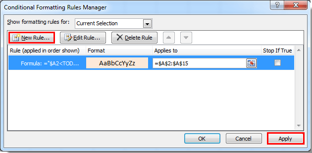
1. Välj intervallet A2: A15 och klicka sedan på Villkorlig formatering > Hantera regler under Hem flik. Se skärmdump:

2. I Reglerhanteraren för villkorlig formatering dialogrutan, klicka på Ny regel knapp.

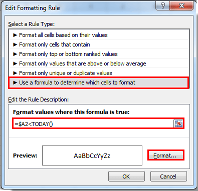
3. I Ny formateringsregel dialogrutan måste du:

1). Välj Använd en formel för att bestämma vilka celler som ska formateras i Välj en regeltyp sektion;

2). För formatera datum äldre än idag, vänligen kopiera och klistra in formeln = $ A2 i Formatera värden där denna formel är sann låda;

För formatera framtida datum, använd denna formel = $ A2> I DAG ();

3). Klicka på bildad knapp. Se skärmdump:

4. I Formatera celler dialogrutan, ange formatet för förfallodatum eller framtida datum och klicka sedan på OK knapp.

5. Sedan återgår den till Reglerhanteraren för villkorlig formatering dialog ruta. Och formateringsregeln för förfallodatum skapas. Om du vill tillämpa regeln nu klickar du på Ansök knapp.

6. Men om du vill tillämpa regeln för förfallodatum och framtida datumregel, skapa en ny regel med formel för framtida formatering av datum genom att upprepa stegen ovan från 2 till 4.

7. När den återgår till Reglerhanteraren för villkorlig formatering dialogrutan igen kan du se att de två reglerna visas i rutan, klicka på OK för att starta formateringen.

Då kan du se de datum som är äldre än idag och datumet som är större än idag har formaterats.

Enkelt villkorligt format varje n rad i valet:

Kutools för Excel's Alternativ rad- / kolumnskuggning verktyget hjälper dig att enkelt lägga till villkorlig formatering till varje n rad i Excel-val.
Ladda ner hela funktionen 30-dagars gratis spår av Kutools för Excel nu!


Relaterade artiklar:

Bästa kontorsproduktivitetsverktyg

🤖 Kutools AI Aide: Revolutionera dataanalys baserat på: Intelligent utförande   |  Generera kod  |  Skapa anpassade formler  |  Analysera data och generera diagram  |  Anropa Kutools funktioner.
Populära funktioner: Hitta, markera eller identifiera dubbletter   |  Ta bort tomma rader   |  Kombinera kolumner eller celler utan att förlora data   |   Rund utan formel ...
Superuppslag: Flera kriterier VLookup    VLookup med flera värden  |   VSök över flera ark   |   Fuzzy Lookup ....
Avancerad rullgardinslista: Skapa snabbt en rullgardinslista   |  Beroende rullgardinslista   |  Flervals-rullgardinslista ....
Kolumnhanterare: Lägg till ett specifikt antal kolumner  |  Flytta kolumner  |  Växla synlighetsstatus för dolda kolumner  |  Jämför intervall och kolumner ...
Utvalda funktioner: Rutnätsfokus   |  Designvy   |   Stor formelbar    Arbetsbok & Bladhanterare   |  Resursbibliotek (Automatisk text)   |  Datumväljare   |  Kombinera arbetsblad   |  Kryptera/Dekryptera celler    Skicka e-postmeddelanden efter lista   |  Superfilter   |   Specialfilter (filtrera fet/kursiv/genomstruken...) ...
Topp 15 verktygssatser12 text verktyg (lägga till text, Ta bort tecken, ...)   |   50+ Diagram Typer (Gantt Chart, ...)   |   40+ Praktiskt Formler (Beräkna ålder baserat på födelsedag, ...)   |   19 Införande verktyg (Infoga QR-kod, Infoga bild från sökväg, ...)   |   12 Konvertering verktyg (Siffror till ord, Valutaväxling, ...)   |   7 Slå ihop och dela verktyg (Avancerade kombinera rader, Dela celler, ...)   |   ... och mer

Uppgradera dina Excel-färdigheter med Kutools för Excel och upplev effektivitet som aldrig förr. Kutools för Excel erbjuder över 300 avancerade funktioner för att öka produktiviteten och spara tid.  Klicka här för att få den funktion du behöver mest...

Beskrivning


Fliken Office ger ett flikgränssnitt till Office och gör ditt arbete mycket enklare

  • Aktivera flikredigering och läsning i Word, Excel, PowerPoint, Publisher, Access, Visio och Project.
  • Öppna och skapa flera dokument i nya flikar i samma fönster, snarare än i nya fönster.
  • Ökar din produktivitet med 50 % och minskar hundratals musklick för dig varje dag!
Comments (24)
No ratings yet. Be the first to rate!
This comment was minimized by the moderator on the site
I want to highlight a cell if:
1. today's date is greater than the date in another cell or blank (=TODAY()>'APM Tracker'P14) AND ALSO;
2. If the date in P15 is greater than P14 same highlight color AND ALSO;
3. If the date in P15 is less than P14 I do not want the highlight
This comment was minimized by the moderator on the site
Hey All,

I want to get only past due dates in the particular column. Instead of highlighting the cells with color i need the dates to be picked in the column

Any solution for this....
This comment was minimized by the moderator on the site
Alright, I read through this thread and did not see this question asked/answered. I have a column of future dates. I would like to add conditional formatting to flag that date exactly 30 days before (1st color "Hey you should get this done its due in 30 day's") and 7 days ( 2nd color "You procrastinated and now you have 7 days to complete this"). Any help here?
This comment was minimized by the moderator on the site
Hi Michael,
I am not sure I understand your question clearly. If you want to hight the date which is 30 days and 7 days from today. Please use the following formulas to create two formula rules with different highlighted colors:
=D9=TODAY()+30
=D9=TODAY()+7

https://www.extendoffice.com/images/stories/comments/comment-picture-zxm/conditional-formatting.png
If this is not what you need, please attach a screenshot of your data here.
This comment was minimized by the moderator on the site
To ignore cells that have blanks try this:

=AND($A2<>"",$A2<TODAY())

This assumes the cell you have selected is A2 (change this to whatever cell you have currently selected)
To copy this to the applicable cells, change the "Applies to" to the cell range you need.
This comment was minimized by the moderator on the site
Hi Andy Campbell,
Thank you for sharing.
This comment was minimized by the moderator on the site
Hi
I am trying to use condition formatting to allow a cell to be highlighted when an item is past due based on different turn around times (TAT). I have a column with a submitted date which is then used with the #of days from the TAT to automatically give the due date. Using the following formula, =IF(OR(E3="",A3=""),"",DATE(YEAR(A3),MONTH(A3),DAY(A3)+E3))
The condition formatting currently used is "cell value < today()" applies to +$G:$G.
What I would like to do is use the stop if rule to stop the condition formatting if the date entered in column "H" is < or = to todays date.
Thanks Michelle
This comment was minimized by the moderator on the site
if i want highlight the due date with the conditional : today less or equal 30 days from due date
This comment was minimized by the moderator on the site
I am trying to create conditional formatting that will highlight rows older than 14 days in yellow and highlight rows older than 21 days in red. My date column starts in A2, I have the following rules applied, but only yellow is highlighting and just the date column, not the entire row. Can you help? Scott

1. =ISBLANK(A2)=TRUE
2. =A2<TODAY()-14
3. =A2<TODAY()-21
This comment was minimized by the moderator on the site
I want to ignore blank cells which doesn't have a date i.e I do not want blank cells to be highlighted when I am comparing dates<Today(). Please help
This comment was minimized by the moderator on the site
Hi Madhu,
The first method in this artice can help you solve the problem. Please have a try.
https://www.extendoffice.com/documents/excel/2499-excel-conditional-formatting-ignore-blank-zero.html
This comment was minimized by the moderator on the site
1 colum has the dates in it i want another colum to change colour when this formula is applied.

any ideas?
This comment was minimized by the moderator on the site
Hi grant,
Supposing you want to change the cell color in column B based on dates in column A, please select the column B cells (such as B2:B21), and apply the conditional formatting function with the above formulas =$A2>Today() or =$A2<Today().
This comment was minimized by the moderator on the site
Hello! can anyone help me?

I have =TODAY() formula in A1 and need 3 more rules to work as per below

rule 1 all dates 8 to 14 days older than today

rule 2 : all dates older 14 to 30 days than today

rule 3: all dates 31 or more days older than today
This comment was minimized by the moderator on the site
it should be something like this:

if(*cell*+8>Today();if(*cell*+14<Today();"8-14 from today";"N/A"))
There are no comments posted here yet
Load More
Please leave your comments in English
Posting as Guest
×
Rate this post:
0   Characters
Suggested Locations