Hur VLOOKUP och returnera flera motsvarande värden horisontellt i Excel?

Som standard kan VLOOKUP-funktionen returnera flera motsvarande värden på den vertikala nivån i Excel, i vissa fall kanske du vill returnera flera värden på horisontell nivå enligt skärmbilden nedan. Här kommer jag att berätta en formel som kan lösa denna uppgift.
VLOOKUP och returnera flera värden horisontellt

VLOOKUP och returnera flera värden horisontellt

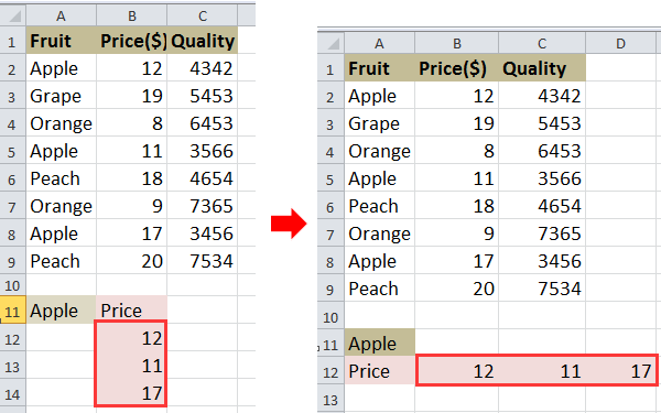
Till exempel, du har ett urval av data som visas nedan, och du vill SE UPP Apples priser.

1. Välj en cell och skriv den här formeln =INDEX($B$2:$B$9, SMALL(IF($A$11=$A$2:$A$9, ROW($A$2:$A$9)-ROW($A$2)+1), COLUMN(A1))) och tryck sedan på Skift + Ctrl + Enter och dra autofyllhandtaget åt höger för att tillämpa denna formel tills #OGILTIGT! visas. Se skärmdump:

2. Ta sedan bort #NUM!. Se skärmdump:

Dricks: I formeln ovan är B2:B9 kolumnintervallet som du vill returnera värdena i, A2:A9 är kolumnintervallet som uppslagsvärdet finns i, A11 är uppslagsvärdet, A1 är den första cellen i ditt dataintervall , A2 är den första cellen i kolumnintervallet som du slår upp värdet i.

Om du vill returnera flera värden vertikalt kan du läsa den här artikeln Hur söker jag upp värden i flera motsvarande värden i Excel?

Kombinera enkelt flera ark / arbetsbok i ett ark eller arbetsbok

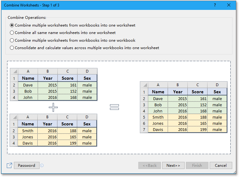
Att kombinera flera ark eller arbetsböcker till ett ark eller arbetsbok kan vara snedigt i Excel, men med Kombinera funktion i Kutools för Excel, du kan kombinera sammanfoga dussintals ark / arbetsböcker till ett ark eller arbetsbok, du kan också konsolidera arken i ett med flera klick.  Klicka för en 30 dagars gratis provperiod med alla funktioner!

Kutools för Excel: med mer än 300 praktiska Excel-tillägg, gratis att prova utan begränsning på 30 dagar.

Bästa kontorsproduktivitetsverktyg

🤖	Kutools AI Aide: Revolutionera dataanalys baserat på: Intelligent utförande   |  Generera kod  |  Skapa anpassade formler  |  Analysera data och generera diagram  |  Anropa Kutools funktioner.
	Populära funktioner: Hitta, markera eller identifiera dubbletter   |  Ta bort tomma rader   |  Kombinera kolumner eller celler utan att förlora data   |   Rund utan formel ...
	Superuppslag: Flera kriterier VLookup  |   VLookup med flera värden  |   VSök över flera ark   |   Fuzzy Lookup ....
	Avancerad rullgardinslista: Skapa snabbt en rullgardinslista   |  Beroende rullgardinslista   |  Flervals-rullgardinslista ....
	Kolumnhanterare: Lägg till ett specifikt antal kolumner  |  Flytta kolumner  |  Växla synlighetsstatus för dolda kolumner  |  Jämför intervall och kolumner ...
	Utvalda funktioner: Rutnätsfokus   |  Designvy   |   Stor formelbar   |  Arbetsbok & Bladhanterare   |  Resursbibliotek (Automatisk text)   |  Datumväljare   |  Kombinera arbetsblad   |  Kryptera/Dekryptera celler   |  Skicka e-postmeddelanden efter lista   |  Superfilter   |   Specialfilter (filtrera fet/kursiv/genomstruken...) ...
	Topp 15 verktygssatser:  12 text verktyg (lägga till text, Ta bort tecken, ...)   |   50+ Diagram Typer (Gantt Chart, ...)   |   40+ Praktiskt Formler (Beräkna ålder baserat på födelsedag, ...)   |   19 Införande verktyg (Infoga QR-kod, Infoga bild från sökväg, ...)   |   12 Konvertering verktyg (Siffror till ord, Valutaväxling, ...)   |   7 Slå ihop och dela verktyg (Avancerade kombinera rader, Dela celler, ...)   |   ... och mer

Uppgradera dina Excel-färdigheter med Kutools för Excel och upplev effektivitet som aldrig förr. Kutools för Excel erbjuder över 300 avancerade funktioner för att öka produktiviteten och spara tid.  Klicka här för att få den funktion du behöver mest...

Läs mer... Gratis nedladdning...

---

Fliken Office ger ett flikgränssnitt till Office och gör ditt arbete mycket enklare

• Aktivera flikredigering och läsning i Word, Excel, PowerPoint, Publisher, Access, Visio och Project.
• Öppna och skapa flera dokument i nya flikar i samma fönster, snarare än i nya fönster.
• Ökar din produktivitet med 50 % och minskar hundratals musklick för dig varje dag!

Läs mer... Gratis nedladdning...