Hur döljer man bara en del av cellvärdet i Excel?

Om du antar att du har ett ark med allmän information om personalen, men en del är privata som personnummer. Nu vill du dölja en del av dessa personnummer som visas nedan på skärmdumpen, hur kan du snabbt lösa det?

Dölj personnummer med Format Cells

Dölj text eller nummer delvis med formler

Dölj personnummer med Format Cells

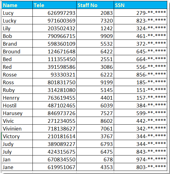
För att dölja en del av personnummer i Excel kan du använda Formatceller för att lösa det.

1. Markera numren som du vill dölja delvis och högerklicka för att välja Formatera celler från snabbmenyn. Se skärmdump:

2. Sedan i Formatera celler dialog, klicka Antal fliken och välj Custom från Kategori och gå till det här 000 ,, "- ** - ****" i Typ rutan i höger avsnitt. Se skärmdump:

3. klick OK, nu har delnummer du valt döljts.

AnmärkningarRound det kommer att runda upp siffran om det fjärde numret är större än eller eaqul till 5.

Dölj text eller nummer delvis med formler

Med ovanstående metod kan du bara dölja delnummer, om du vill dölja delnummer eller texter kan du göra som nedan:

Här döljer vi de första fyra numren i passnumret.

Välj en tom cell bredvid passnumret, till exempel F22, ange denna formel = "****" & HÖGER (E22,5)och dra sedan autofyllhandtaget över cellen du behöver för att tillämpa denna formel.

Dricks:

Om du vill dölja de fyra senaste siffrorna, använd den här formeln, = VÄNSTER (H2,5) & "****"

Om du vill dölja de tre mellersta siffrorna, använd det här = VÄNSTER (H2,3) & "***" & HÖGER (H2,3)

Bästa kontorsproduktivitetsverktyg

🤖	Kutools AI Aide: Revolutionera dataanalys baserat på: Intelligent utförande   |  Generera kod  |  Skapa anpassade formler  |  Analysera data och generera diagram  |  Anropa Kutools funktioner.
	Populära funktioner: Hitta, markera eller identifiera dubbletter   |  Ta bort tomma rader   |  Kombinera kolumner eller celler utan att förlora data   |   Rund utan formel ...
	Superuppslag: Flera kriterier VLookup  |   VLookup med flera värden  |   VSök över flera ark   |   Fuzzy Lookup ....
	Avancerad rullgardinslista: Skapa snabbt en rullgardinslista   |  Beroende rullgardinslista   |  Flervals-rullgardinslista ....
	Kolumnhanterare: Lägg till ett specifikt antal kolumner  |  Flytta kolumner  |  Växla synlighetsstatus för dolda kolumner  |  Jämför intervall och kolumner ...
	Utvalda funktioner: Rutnätsfokus   |  Designvy   |   Stor formelbar   |  Arbetsbok & Bladhanterare   |  Resursbibliotek (Automatisk text)   |  Datumväljare   |  Kombinera arbetsblad   |  Kryptera/Dekryptera celler   |  Skicka e-postmeddelanden efter lista   |  Superfilter   |   Specialfilter (filtrera fet/kursiv/genomstruken...) ...
	Topp 15 verktygssatser:  12 text verktyg (lägga till text, Ta bort tecken, ...)   |   50+ Diagram Typer (Gantt Chart, ...)   |   40+ Praktiskt Formler (Beräkna ålder baserat på födelsedag, ...)   |   19 Införande verktyg (Infoga QR-kod, Infoga bild från sökväg, ...)   |   12 Konvertering verktyg (Siffror till ord, Valutaväxling, ...)   |   7 Slå ihop och dela verktyg (Avancerade kombinera rader, Dela celler, ...)   |   ... och mer

Uppgradera dina Excel-färdigheter med Kutools för Excel och upplev effektivitet som aldrig förr. Kutools för Excel erbjuder över 300 avancerade funktioner för att öka produktiviteten och spara tid.  Klicka här för att få den funktion du behöver mest...

Läs mer... Gratis nedladdning...

---

Fliken Office ger ett flikgränssnitt till Office och gör ditt arbete mycket enklare

• Aktivera flikredigering och läsning i Word, Excel, PowerPoint, Publisher, Access, Visio och Project.
• Öppna och skapa flera dokument i nya flikar i samma fönster, snarare än i nya fönster.
• Ökar din produktivitet med 50 % och minskar hundratals musklick för dig varje dag!

Läs mer... Gratis nedladdning...