Hoppa till huvudinnehåll

Hur visar jag det första objektet i listrutan istället för tomt?

nedrullningsdokument för doc som standard till topp 1

Listrutan i ett kalkylblad kan hjälpa oss att göra datainmatning enklare, vi behöver bara välja objekten utan att skriva dem en efter en. Men någon gång, när du klickar på rullgardinsmenyn, hoppar den till de tomma objekten först i stället för det första dataobjektet som följande skärmdump visas, detta kan bero på att radera källdata i slutet av listan. Det kan vara irriterande att du måste bläddra tillbaka till toppen av en lång lista för varje tom datavalideringscell. Den här artikeln kommer jag att prata om hur man alltid visar det första objektet i listrutan.

Visa det första objektet i listrutan istället för tomt med funktionen Data Validation

Visa automatiskt det första objektet i listrutan istället för tomt med VBA-kod


pil blå höger bubbla Visa det första objektet i listrutan istället för tomt med funktionen Data Validation

För att uppnå detta jobb behöver du faktiskt bara använda en specifik formel när du skapar en rullgardinslista, gör så här:

1. Markera cellerna där du vill infoga listrutan och klicka Data > Datagransknings > Datagransknings, se skärmdump:

nedrullningsdokument för doc som standard till topp 2

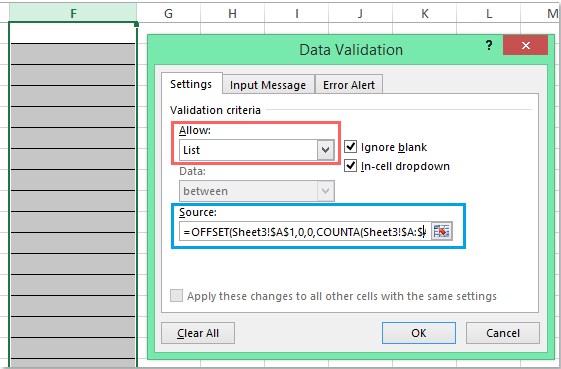
2. I poppade ut Datagransknings under dialogrutan Inställningar fliken, välj Lista från Tillåt avsnitt och ange sedan denna formel: = OFFSET (Sheet3! $ A $ 1,0,0, COUNTA (Sheet3! $ A: $ A) -1,1) i Källa textruta, se skärmdump:

Anmärkningar: I denna formel, Sheet3 är kalkylbladet innehåller källdatalistan, och A1 är det första cellvärdet i listan.

nedrullningsdokument för doc som standard till topp 3

3. Klicka sedan OK -knappen, nu när du klickar på rullgardinsmenyerna visas det första dataobjektet alltid överst om det finns cellvärden som raderas i slutet av källdata, se skärmdump:

nedrullningsdokument för doc som standard till topp 4


pil blå höger bubbla Visa automatiskt det första objektet i listrutan istället för tomt med VBA-kod

Här kan jag också införa en VBA-kod som kan hjälpa dig att visa det första objektet i rullgardinslistan automatiskt när du klickar på datavalideringscellerna.

1. När du har infogat rullgardinsmenyn, välj fliken kalkylblad som innehåller rullgardinsmenyn och högerklicka för att välja Visa kod från snabbmenyn för att gå till Microsoft Visual Basic för applikationer och kopiera och klistra sedan in följande kod i modulen:

VBA-kod: Visa automatiskt det första dataobjektet i listrutan:

Private Sub Worksheet_SelectionChange(ByVal Target As Range)
'Updateby Extendoffice 20160725
    Dim xFormula As String
    On Error GoTo Out:
    xFormula = Target.Cells(1).Validation.Formula1
    If Left(xFormula, 1) = "=" Then
        Target.Cells(1) = Range(Mid(xFormula, 1)).Cells(1).Value
    End If
Out:
End Sub

nedrullningsdokument för doc som standard till topp 5

2. Spara och stäng sedan kodfönstret, och nu, när du klickar på rullgardinsmenyn, kommer det första dataobjektet att visas på en gång.

Bästa kontorsproduktivitetsverktyg

🤖 Kutools AI Aide: Revolutionera dataanalys baserat på: Intelligent utförande   |  Generera kod  |  Skapa anpassade formler  |  Analysera data och generera diagram  |  Anropa Kutools funktioner.
Populära funktioner: Hitta, markera eller identifiera dubbletter   |  Ta bort tomma rader   |  Kombinera kolumner eller celler utan att förlora data   |   Rund utan formel ...
Superuppslag: Flera kriterier VLookup    VLookup med flera värden  |   VSök över flera ark   |   Fuzzy Lookup ....
Avancerad rullgardinslista: Skapa snabbt en rullgardinslista   |  Beroende rullgardinslista   |  Flervals-rullgardinslista ....
Kolumnhanterare: Lägg till ett specifikt antal kolumner  |  Flytta kolumner  |  Växla synlighetsstatus för dolda kolumner  |  Jämför intervall och kolumner ...
Utvalda funktioner: Rutnätsfokus   |  Designvy   |   Stor formelbar    Arbetsbok & Bladhanterare   |  Resursbibliotek (Automatisk text)   |  Datumväljare   |  Kombinera arbetsblad   |  Kryptera/Dekryptera celler    Skicka e-postmeddelanden efter lista   |  Superfilter   |   Specialfilter (filtrera fet/kursiv/genomstruken...) ...
Topp 15 verktygssatser12 text verktyg (lägga till text, Ta bort tecken, ...)   |   50+ Diagram Typer (Gantt Chart, ...)   |   40+ Praktiskt Formler (Beräkna ålder baserat på födelsedag, ...)   |   19 Införande verktyg (Infoga QR-kod, Infoga bild från sökväg, ...)   |   12 Konvertering verktyg (Siffror till ord, Valutaväxling, ...)   |   7 Slå ihop och dela verktyg (Avancerade kombinera rader, Dela celler, ...)   |   ... och mer

Uppgradera dina Excel-färdigheter med Kutools för Excel och upplev effektivitet som aldrig förr. Kutools för Excel erbjuder över 300 avancerade funktioner för att öka produktiviteten och spara tid.  Klicka här för att få den funktion du behöver mest...

Beskrivning


Fliken Office ger ett flikgränssnitt till Office och gör ditt arbete mycket enklare

  • Aktivera flikredigering och läsning i Word, Excel, PowerPoint, Publisher, Access, Visio och Project.
  • Öppna och skapa flera dokument i nya flikar i samma fönster, snarare än i nya fönster.
  • Ökar din produktivitet med 50 % och minskar hundratals musklick för dig varje dag!
Comments (10)
No ratings yet. Be the first to rate!
This comment was minimized by the moderator on the site
=OFFSET(Sheet3!$A$1,0,0,COUNTA(Sheet3!$A:$A)+2-1,1) I added +2 to the equation and that worked for me.
This comment was minimized by the moderator on the site
For the VDA code, how can I have only a certain cell range show the first item in the drop down list? Thank you in advance.
This comment was minimized by the moderator on the site
Hi, Akrupa,To solve your problem, maybe the following VBA code can help you:

<div data-tag="code">Private Sub Worksheet_SelectionChange(ByVal Target As Range)
'Updateby Extendoffice 20211206
Dim xFormula As String
Dim xRg As Range
Dim xStr As String
Dim xIndex As Integer
xIndex = 2 'Here indicates the cell number of the original data,for example,the original data is A1:A10, to display the A2 cell value, please write 2 here.
On Error GoTo Out:
xFormula = Target.Cells(1).Validation.Formula1
If Left(xFormula, 1) = "=" Then
If Target.Value <> "" Then Exit Sub
xStr = Mid(xFormula, 2)
Set xRg = Application.Range(xStr)
Target.Cells(1) = xRg.Cells(xIndex).Value
End If
Out:
End Sub
Please try, hope it can help you!
This comment was minimized by the moderator on the site
Better but not quite. Using the =OFFSET(Sheet3!$A$1,0,0,COUNTA(Sheet3!$A:$A)-1,1) method eliminates the blanks but still starts you at the bottom of the very long list. I want it to start at the top of the list.
This comment was minimized by the moderator on the site
Once again, you save the day! Thanks!
This comment was minimized by the moderator on the site
Doesn't work for me. I keep getting an error message that says, "There's a problem with this formula. Not trying to type a formula? When the first character is an equal (+) or minus (-) sign, Exel thinks it's a formula.... To get around this, type an apostrophe (') first..."
This comment was minimized by the moderator on the site
Hello!

How can I set a data validation list such that if the drop down value in the cell is deleted, the cell will automatically show a default value (i.e. "-Select-")?

For example, I have a worksheet with multiple drop down lists that I want to show a default value of "-Select-" once the sheet is opened. A user will select values from the lists that will impact the result of calculations throughout the entire spreadsheet. A user may accidentally "delete" the cell contents of the lists. If this happens, rather than the cell becoming blank, I want the cell to show a default value of "-Select-". This scenario occurs in multiple random locations throughout the spreadsheet, not just in one localized place.

I was able to find the following VBA code so far, but it only applies the concept over a range, rather than just individual cells that contain drop down lists. The problem with what I have coded so far is that every single blank cell in the range ends up with "-Select-" in it. Some of the lists are in ranges, but some are also scattered throughout the sheet. The problem I'm having with my current code is that every single blank cell in the range ends up with "-Select-" in it. I'm trying to get this to apply over the entire worksheet to ONLY cells that are drop down lists.

Is what I'm trying to accomplish even possible?

Example file can be found here:
https://drive.google.com/file/d/1VoO8VgFs3IJ0ALwqfk0i8gt69UE4vEKW/view?usp=sharing

Example code:

Option Explicit

Private Sub Worksheet_Change(ByVal Target As Range)
Dim cel As Range
' If Target.Cells.Count > 1 Then Exit Sub 'turning this off allows multiple cells to be selected and deleted at the same time
If Not Intersect(Target, Range("f2:p17")) Is Nothing Then
For Each cel In Range("f2:p17")
Application.EnableEvents = False
If IsEmpty(cel.Value) Then cel.Value = "-Select-"
Next cel
End If
Application.EnableEvents = True
End Sub


Thanks in advance!
This comment was minimized by the moderator on the site
How can I set a data validation list such that if the drop down value in the cell is deleted, the cell will automatically show the a default value (i.e. "-Select-")?

For example, I have a worksheet with multiple drop down lists that I want to show a default value of "-Select-" once the sheet is opened. A user will select values from the lists that will impact the result of calculations throughout the entire spreadsheet. A user may accidentally "delete" the cell contents. If this happens, rather than the cell becoming blank, I want the cell to show a default value of "-Select-". This scenario occurs in multiple random locations throughout the spreadsheet, not just in one localized place.

I was able to come up with the following VBA code so far, but I've only figured out how to apply the concept over a range, rather than just cells that contain a drop down list. The problem with what I have coded so far is that every single blank cell in the range ends up with "-Select-" in it.

Option Explicit

Private Sub Worksheet_Change(ByVal Target As Range)
Dim cel As Range
' If Target.Cells.Count > 1 Then Exit Sub
If Not Intersect(Target, Range("f2:p17")) Is Nothing Then
For Each cel In Range("f2:p17")
Application.EnableEvents = False
If IsEmpty(cel.Value) Then cel.Value = "-Select-"
Next cel
End If
Application.EnableEvents = True
End Sub
This comment was minimized by the moderator on the site
select the cell in which you have put the listitem
the range for the listitem is "Opleiding"
in your VBA code:

selection.Value = Range("opleiding").Cells(2, 1)

the result is that the selected item of the listItem is the second item in the range "Opleiding"
This comment was minimized by the moderator on the site
After scroll down select to cells numeric data not come in series only first cell data come select 1,2 different cells and scroll down value not coming 1,2,3,4,5....... only first cell value coming 1,1,1,1,....
There are no comments posted here yet
Please leave your comments in English
Posting as Guest
×
Rate this post:
0   Characters
Suggested Locations