Hoppa till huvudinnehåll

Hur länkar man pivottabelfilter till en viss cell i Excel?

Om du vill länka ett pivottabelfilter till en viss cell och göra pivottabellen filtrerad baserat på cellvärdet kan metoden i den här artikeln hjälpa dig.

Länka pivottabelfiltret till en viss cell med VBA-kod


Länka pivottabelfiltret till en viss cell med VBA-kod

Pivottabellen som du kommer att länka dess filterfunktion till ett cellvärde bör innehålla ett filterfält (namnet på filterfältet spelar en viktig roll i följande VBA-kod).

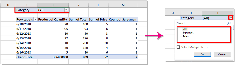
Ta nedanstående pivottabell som ett exempel. Filterfältet i pivottabellen kallas Kategori, och den innehåller två värden ”Kostnader"Och"Försäljning”. Efter att ha kopplat pivottabelfiltret till en cell bör de cellvärden som du kommer att använda för att filtrera pivottabellen vara "Utgifter" och "Försäljning".

1. Välj den cell (här väljer jag cell H6) som du kommer att länka till Pivot Tabells filterfunktion och ange ett av filtervärdena i cellen i förväg.

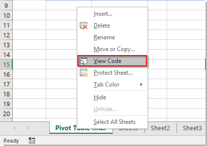
2. Öppna kalkylbladet innehåller pivottabellen som du kommer att länka till cellen. Högerklicka på arkfliken och välj Visa kod från snabbmenyn. Se skärmdump:

3. I Microsoft Visual Basic för applikationer kopiera under VBA-koden till kodfönstret.

VBA-kod: Länk pivottabelfilter till en viss cell

Private Sub Worksheet_Change(ByVal Target As Range)
'Update by Extendoffice 20180702
    Dim xPTable As PivotTable
    Dim xPFile As PivotField
    Dim xStr As String
    On Error Resume Next
    If Intersect(Target, Range("H6")) Is Nothing Then Exit Sub
    Application.ScreenUpdating = False
    Set xPTable = Worksheets("Sheet1").PivotTables("PivotTable2")
    Set xPFile = xPTable.PivotFields("Category")
    xStr = Target.Text
    xPFile.ClearAllFilters
    xPFile.CurrentPage = xStr
    Application.ScreenUpdating = True
End Sub

Anmärkningar:

1) "Sheet1”Är namnet på det öppnade kalkylbladet.
2) "Pivottabell2”Är namnet på pivottabellen, du kommer att länka dess filterfunktion till en cell.
3) Filtreringsfältet i pivottabellen kallas "Kategori".
4) Den refererade cellen är H6. Du kan ändra dessa variabla värden baserat på dina behov.

4. tryck på andra + Q för att stänga Microsoft Visual Basic för applikationer fönster.

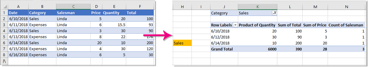
Nu är filterfunktionen i pivottabellen kopplad till cell H6.

Uppdatera cellen H6, sedan filtreras motsvarande data i pivottabellen ut baserat på det befintliga värdet. Se skärmdump:

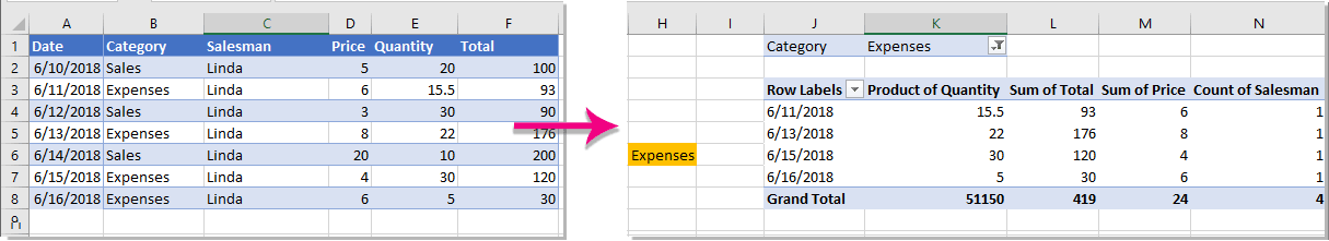
När du ändrar cellvärdet ändras de filtrerade data i pivottabellen automatiskt. Se skärmdump:


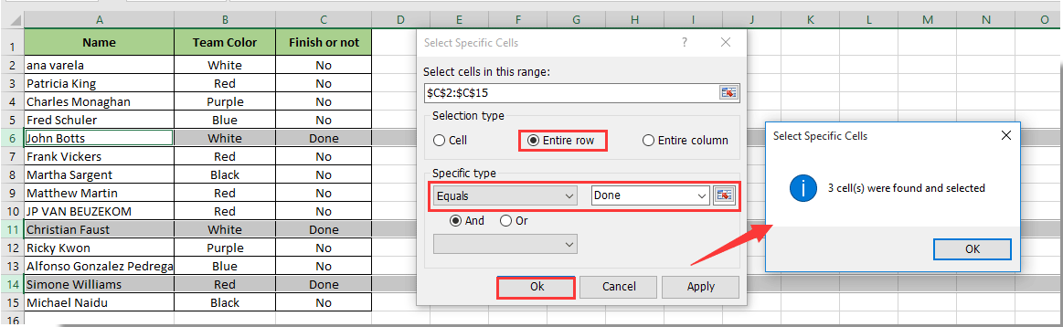
Välj enkelt hela rader baserat på cellvärde i en certian-kolumn:

Smakämnen Välj specifika celler nytta av Kutools för Excel kan hjälpa dig att snabbt välja hela rader baserat på cellvärde i en certian-kolumn i Excel som visas nedan. När du har valt alla rader baserat på cellvärde kan du manuellt flytta eller kopiera dem till en ny plats som du behöver i Excel.
Ladda ner och prova nu! (30 dagars gratis spår)


Relaterade artiklar:

Bästa kontorsproduktivitetsverktyg

🤖 Kutools AI Aide: Revolutionera dataanalys baserat på: Intelligent utförande   |  Generera kod  |  Skapa anpassade formler  |  Analysera data och generera diagram  |  Anropa Kutools funktioner.
Populära funktioner: Hitta, markera eller identifiera dubbletter   |  Ta bort tomma rader   |  Kombinera kolumner eller celler utan att förlora data   |   Rund utan formel ...
Superuppslag: Flera kriterier VLookup    VLookup med flera värden  |   VSök över flera ark   |   Fuzzy Lookup ....
Avancerad rullgardinslista: Skapa snabbt en rullgardinslista   |  Beroende rullgardinslista   |  Flervals-rullgardinslista ....
Kolumnhanterare: Lägg till ett specifikt antal kolumner  |  Flytta kolumner  |  Växla synlighetsstatus för dolda kolumner  |  Jämför intervall och kolumner ...
Utvalda funktioner: Rutnätsfokus   |  Designvy   |   Stor formelbar    Arbetsbok & Bladhanterare   |  Resursbibliotek (Automatisk text)   |  Datumväljare   |  Kombinera arbetsblad   |  Kryptera/Dekryptera celler    Skicka e-postmeddelanden efter lista   |  Superfilter   |   Specialfilter (filtrera fet/kursiv/genomstruken...) ...
Topp 15 verktygssatser12 text verktyg (lägga till text, Ta bort tecken, ...)   |   50+ Diagram Typer (Gantt Chart, ...)   |   40+ Praktiskt Formler (Beräkna ålder baserat på födelsedag, ...)   |   19 Införande verktyg (Infoga QR-kod, Infoga bild från sökväg, ...)   |   12 Konvertering verktyg (Siffror till ord, Valutaväxling, ...)   |   7 Slå ihop och dela verktyg (Avancerade kombinera rader, Dela celler, ...)   |   ... och mer

Uppgradera dina Excel-färdigheter med Kutools för Excel och upplev effektivitet som aldrig förr. Kutools för Excel erbjuder över 300 avancerade funktioner för att öka produktiviteten och spara tid.  Klicka här för att få den funktion du behöver mest...

Beskrivning


Fliken Office ger ett flikgränssnitt till Office och gör ditt arbete mycket enklare

  • Aktivera flikredigering och läsning i Word, Excel, PowerPoint, Publisher, Access, Visio och Project.
  • Öppna och skapa flera dokument i nya flikar i samma fönster, snarare än i nya fönster.
  • Ökar din produktivitet med 50 % och minskar hundratals musklick för dig varje dag!
Comments (38)
No ratings yet. Be the first to rate!
This comment was minimized by the moderator on the site
Hi,
This code worked perfectly on the pivot table, but I also want to link a filter to a cell value on a Table. Is there code for this? Please help :)
This comment was minimized by the moderator on the site
if my column in pivot table is date this code not working, can some one help me please
This comment was minimized by the moderator on the site
Можно ли сослаться вместо ячейки H6 на ячейку на другом листе? как это сделать? подскажите пожалуйста.
This comment was minimized by the moderator on the site
Hi Алексей,

You don't need to modify the code, just add the VBA code to the worksheet of the cell you want to reference.
For example, if you want to filter a pivot table named "PivotTable1" in Sheet2 based on the value of cell H6 in Sheet3, please right click the Sheet3 worksheet tab, click View Code from the right-clicking menu, and then add the code to the Sheet3 (Code) window.
This comment was minimized by the moderator on the site
Как сделать чтобы сводная таблица применяла сразу 2 фильтра из 2хразных ячеек? а не 1 как в примере?
This comment was minimized by the moderator on the site
Hi Алексей,

Please check if the VBA code in this comment #38754 can help.
This comment was minimized by the moderator on the site
find these and change it in Array(),Intersect(), Worksheets(), PivotFields()

PivotTable1
PivotTable2
PivotTable3
PivotTable4
H1
SheetName
FieldName


Private Sub Worksheet_Change(ByVal Target As Range)
'Update by Extendoffice 20180702
    Dim xPTable As PivotTable
    Dim xPFile As PivotField
    Dim xPTabled As PivotTable
    Dim xPFiled As PivotField
    Dim xStr As String
    On Error Resume Next
    '리스트 만들기
    Dim listArray() As Variant
    listArray = Array("PivotTable1", "PivotTable2", "PivotTable3", "PivotTable4")
    If Intersect(Target, Range("H1")) Is Nothing Then Exit Sub
    Application.ScreenUpdating = False
    For i = 0 To UBound(listArray)
        Set xPTable = Worksheets("SheetName").PivotTables(listArray(i))
        Set xPFile = xPTable.PivotFields("FieldName")
        'MsgBox (listArray(i))
        xStr = Target.Text
        xPFile.ClearAllFilters
        xPFile.CurrentPage = xStr
    Next
        Application.ScreenUpdating = True
End Sub
This comment was minimized by the moderator on the site
Hello,

This code works perfectly. However I am not able to get the code to update the pivot table automatically. The target value for me is a formula (=DATE(D18,..,..)) which changes depending on what is selected at D18. For it to update the pivot table i have to double click the target cell and hit enter. Is there a way around it?

Thank you
This comment was minimized by the moderator on the site
Hello ST,
Suppose your target value is in H6 and it changes depending on the value in D18. To filter a pivot table based on this target value. The following VBA code can help. Please give it a try.
Private Sub Worksheet_Change(ByVal Target As Range)
'Updated by Extendoffice 2022/07/22
Dim xPTable As PivotTable
Dim xPFile As PivotField
Dim xStr As String
Dim xBoolean As Boolean
Dim xItsRG As Range
Dim xDDs As Range
Dim xDs As Range
On Error Resume Next

xBoolean = False
Set xRg = Range("h6")

Set xItsRG = Intersect(Target, xRg)
Set xDDs = Intersect(Target.DirectDependents, xRg)
Set xDs = Intersect(Target.Dependents, xRg)
If Not (xItsRG Is Nothing) Then
    xBoolean = True
ElseIf Not (xDDs Is Nothing) Then
    xBoolean = True
ElseIf Not (xDs Is Nothing) Then
    xBoolean = True
End If


If Not xBoolean Then Exit Sub

Application.ScreenUpdating = False
Set xPTable = Worksheets("Sheet1").PivotTables("Pivot Table 1")
Set xPFile = xPTable.PivotFields("Category")
xStr = Target.Text
xPFile.ClearAllFilters
xPFile.CurrentPage = xStr
Application.ScreenUpdating = True

End Sub
This comment was minimized by the moderator on the site
Hello Crysal,

I added a line on the code : Dim xRg As Range

The code doesn't automatically reset the dates when the target is changed. I have an excel file replicating what I am trying to do, I a not able to add attachments on this website though. D3 (target = DATE(A15,B15,C15)) has an equation linked to A15, B15 and C15. When any value on A15, B15 and C15 is changed the pivot table resets to no filter. Could you help me out on this?
This comment was minimized by the moderator on the site
Hi ST,
I don't quite understand what you mean. In your case, the value of target cell D3 is used to filter the pivot table. The formula in the target cell D3 references the values of cells A15, B15 and C15, which will change according to the values in the reference cells. When any value on A15, B15 and C15 is changed, the pivot table will be automatically filtered if the value in the target cell meets the filter conditions of the pivot table. If the value in the target cell does not meet the pivot table's filtering criteria, the pivot table will be automatically reset to no filtering.
This comment was minimized by the moderator on the site
I’m not sure if there is a way to share an excel file with you. If my target value, which is a date, changes according to changes in other cells. I have to double click on the target cell and hit enter (like you would after entering a formula in a cell) to update the pivot table
This comment was minimized by the moderator on the site
Hi Sagar T,
The code has been updated. Please give it a try. Thanks for your feedback.
Don't forget to change the names of the worksheet, pivot table and the filter in the code. Or you can download the following uploaded workbook for testing.

Private Sub Worksheet_Change(ByVal Target As Range)
'Updated by Extendoffice 20220805
Dim xPTable As PivotTable
Dim xPFile As PivotField
Dim xStr As String
Dim xBoolean As Boolean
Dim xItsRG As Range
Dim xDDs As Range
Dim xDs As Range
On Error Resume Next

xBoolean = False
Set xRg = Range("D3")

Set xItsRG = Intersect(Target, xRg)
Set xDDs = Intersect(Target.DirectDependents, xRg)
Set xDs = Intersect(Target.Dependents, xRg)
If Not (xItsRG Is Nothing) Then
    xBoolean = True
ElseIf Not (xDDs Is Nothing) Then
    xBoolean = True
ElseIf Not (xDs Is Nothing) Then
    xBoolean = True
End If


If Not xBoolean Then Exit Sub
xStr = Format(xRg.Text, "m/d/yyyy")
Application.ScreenUpdating = False
Set xPTable = Worksheets("Sheet2").PivotTables("PivotTable1")
Set xPFile = xPTable.PivotFields("Date")
xPFile.ClearAllFilters
xPFile.CurrentPage = xStr
Application.ScreenUpdating = True

End Sub
This comment was minimized by the moderator on the site
Hello,

The code works fine for me. However I am not able to get the pivot table to update the filter target automatically. The target in my case is a formula [DATE(D18,S14,C18)]. The code only works when I double click the target cell and hit enter.

Thank you
This comment was minimized by the moderator on the site
Hi Justin,

This has worked perfectly, however, I am wondering if this rule can be applied to multiple PivotTables within the same sheet?

Thanks,
James
This comment was minimized by the moderator on the site
Change Values in Array(), Worksheets() and Intersect()


**Find these and change it**
SheetName
E1
PivotTable1
PivotTable2
PivotTable3


Private Sub Worksheet_Change(ByVal Target As Range)
'Update by Extendoffice 20180702
Dim xPTable As PivotTable
Dim xPFile As PivotField

Dim xPTabled As PivotTable
Dim xPFiled As PivotField

Dim xStr As String


On Error Resume Next

'리스트 만들기
Dim listArray() As Variant
listArray = Array("PivotTable1", "PivotTable2", "PivotTable3")


If Intersect(Target, Range("E1")) Is Nothing Then Exit Sub
Application.ScreenUpdating = False

For i = 0 To UBound(listArray)

Set xPTable = Worksheets("SheetName").PivotTables(listArray(i))
Set xPFile = xPTable.PivotFields("Company_ID")

xStr = Target.Text
xPFile.ClearAllFilters
xPFile.CurrentPage = xStr


Next

Application.ScreenUpdating = True


End Sub
This comment was minimized by the moderator on the site
Hi James,

Yes this is possible, code I used for this is (4 pivots and 2 cell references):

Private Sub Worksheet_Change(ByVal Target As Range)
Dim I As Integer
Dim xFilterStr1, xFilterStr2, yFilterstr1, yfilterstr2 As String
On Error Resume Next
If Intersect(Target, Range("O26:P27")) Is Nothing Then Exit Sub

xFilterStr1 = Range("O26").Value
xFilterStr2 = Range("O27").Value
yFilterstr1 = Range("p26").Value
yfilterstr2 = Range("p27").Value
ActiveSheet.PivotTables("Order_Comp_B2C_Crea").PivotFields("Week Number"). _
ActiveSheet.PivotTables("Order_Comp_B2B_Crea").PivotFields("Week Number"). _
ActiveSheet.PivotTables("Order_Comp_B2C_Disp").PivotFields("Week Number"). _
ActiveSheet.PivotTables("Order_Comp_B2B_Disp").PivotFields("Week Number"). _
ClearAllFilters

If xFilterStr1 = "" And xFilterStr2 = "" And yFilterstr1 = "" And yfilterstr2 = "" Then Exit Sub
ActiveSheet.PivotTables("Order_Comp_B2C_Crea").PivotFields("Week Number"). _
ActiveSheet.PivotTables("Order_Comp_B2B_Crea").PivotFields("Week Number"). _
ActiveSheet.PivotTables("Order_Comp_B2C_Disp").PivotFields("Week Number"). _
ActiveSheet.PivotTables("Order_Comp_B2B_Disp").PivotFields("Week Number"). _
EnableMultiplePageItems = True

xCount = ActiveSheet.PivotTables("Order_Comp_B2C_Crea").PivotFields("Week Number").PivotItems.Count
xCount = ActiveSheet.PivotTables("Order_Comp_B2B_Crea").PivotFields("Week Number").PivotItems.Count
yCount = ActiveSheet.PivotTables("Order_Comp_B2C_Disp").PivotFields("Week Number").PivotItems.Count
yCount = ActiveSheet.PivotTables("Order_Comp_B2B_Disp").PivotFields("Week Number").PivotItems.Count

For I = 1 To xCount
If I <> xFilterStr1 And I <> xFilterStr2 Then
ActiveSheet.PivotTables("Order_Comp_B2C_Crea").PivotFields("Week Number").PivotItems(I).Visible = False
ActiveSheet.PivotTables("Order_Comp_B2B_Crea").PivotFields("Week Number").PivotItems(I).Visible = False
Else
ActiveSheet.PivotTables("Order_Comp_B2C_Crea").PivotFields("Week Number").PivotItems(I).Visible = True
ActiveSheet.PivotTables("Order_Comp_B2B_Crea").PivotFields("Week Number").PivotItems(I).Visible = True
End If
Next

For I = 1 To yCount
If I <> yFilterstr1 And I <> yfilterstr2 Then
ActiveSheet.PivotTables("Order_Comp_B2C_Disp").PivotFields("Week Number").PivotItems(I).Visible = False
ActiveSheet.PivotTables("Order_Comp_B2B_Disp").PivotFields("Week Number").PivotItems(I).Visible = False
Else
ActiveSheet.PivotTables("Order_Comp_B2C_Disp").PivotFields("Week Number").PivotItems(I).Visible = True
ActiveSheet.PivotTables("Order_Comp_B2B_Disp").PivotFields("Week Number").PivotItems(I).Visible = True
End If
Next

End Sub
This comment was minimized by the moderator on the site
I used it for a normal excell and it worked.But I could not use it for an olap worksheets. maybe I need to change it a little?
This comment was minimized by the moderator on the site
Hi maziaritib4 TIB,
The method is only avaliable for Microsoft Excel. Sorry for the inconvenience.
This comment was minimized by the moderator on the site
Hi,

Tried to get this working for the column filter but does not seem to work. Do I need an other code for that?

Thanks
This comment was minimized by the moderator on the site
Hi Justin,
Did you get any error prompt? I need to know more specific about your issue.
Before applying the code, don't forget to modify the "name of the sheet", "name of the pivot table", "name of the filter of pivot table" and the cell you want to filter the pivot table based on (see sceenshot).
https://www.extendoffice.com/images/stories/comments/comment-picture-zxm/4.png
This comment was minimized by the moderator on the site
Hi Crystal,

Thanks for your help. Issue is the function is not doing anything for some reason. Some clarification:

Pivot name: Order_Comp_B2C
Sheet Name: Calculation Sheet
Filter name: Week Number (I changed this name from what was "Dispatch Week No" in the data file)
Cell to change: O26 and O27 (this should go in range)

In this pivot, I am trying to get the filter changed for the columns, I have nothing in the filter area in the PivotTable Fields menu.

my code is:

Private Sub Worksheet_Change(ByVal Target As Range)
'Update by Extendoffice 20180702
Dim xPTable As PivotTable
Dim xPFile As PivotField
Dim xStr As String
On Error Resume Next
If Intersect(Target, Range("O26")) Is Nothing Then Exit Sub
Application.ScreenUpdating = False
Set xPTable = Worksheets("Calculation Sheet").PivotTables("Order_Comp_B2C")
Set xPFile = xPTable.PivotFields("Week Number")
xStr = Target.Text
xPFile.ClearAllFilters
xPFile.CurrentPage = xStr
Application.ScreenUpdating = True
End Sub

Thanks,

Justin
This comment was minimized by the moderator on the site
Hi Justin Teeuw,
I have changed the Pivot name, sheet name, filter name and cell to change to the conditions you mentioned above, and tried the VBA code you provided, it works well in my case. See the following GIF or the attached workbook.
Do you mind creating a new workbook and try the code again?
https://www.extendoffice.com/images/stories/comments/comment-picture-zxm/6.gif
This comment was minimized by the moderator on the site
Hi Crystal,

Attached a screenshot of the pivot, the red box is the filter I would like to change based on the cell value.

Preferably I would like to use a range of cells indicating multiple week numbers.

Thanks,

Justin
This comment was minimized by the moderator on the site
Hi Justin Teeuw,
Please try the following VBA code. Hope I can help.

Private Sub Worksheet_Change(ByVal Target As Range)
    'Update by Extendoffice 20220706
    Dim I As Integer
    Dim xFilterStr1, xFilterStr2 As String
    On Error Resume Next
    If Intersect(Target, Range("O26:O27")) Is Nothing Then Exit Sub
    'Application.ScreenUpdating = False
    
    xFilterStr1 = Range("O26").Value
    xFilterStr2 = Range("O27").Value
    ActiveSheet.PivotTables("Order_Comp_B2C").PivotFields("Week Number"). _
        ClearAllFilters
    If xFilterStr1 = "" And xFilterStr2 = "" Then Exit Sub
    ActiveSheet.PivotTables("Order_Comp_B2C").PivotFields("Week Number"). _
        EnableMultiplePageItems = True
    xCount = ActiveSheet.PivotTables("Order_Comp_B2C").PivotFields("Week Number").PivotItems.Count

    For I = 1 To xCount
        If I <> xFilterStr1 And I <> xFilterStr2 Then
            ActiveSheet.PivotTables("Order_Comp_B2C").PivotFields("Week Number").PivotItems(I).Visible = False
        Else
            ActiveSheet.PivotTables("Order_Comp_B2C").PivotFields("Week Number").PivotItems(I).Visible = True
        End If
    Next

    'Application.ScreenUpdating = True
End Sub
This comment was minimized by the moderator on the site
Hi Justin,
Sorry I didn't see the screenshot you attached on the page. Maybe there is some error on the page.
If you still need to solve the problem, email me via . Sorry for the inconvenience.
There are no comments posted here yet
Load More
Please leave your comments in English
Posting as Guest
×
Rate this post:
0   Characters
Suggested Locations