Hoppa till huvudinnehåll

Hur returnerar jag flera matchande värden baserat på ett eller flera kriterier i Excel?

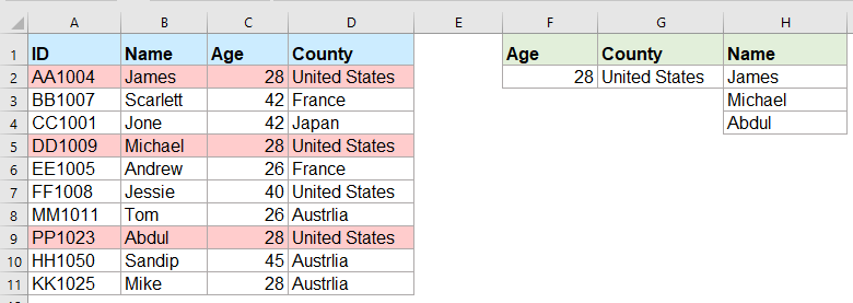
Normalt är det enkelt för de flesta av oss att leta upp ett visst värde och returnera det matchande objektet med hjälp av VLOOKUP-funktionen. Men har du någonsin försökt att returnera flera matchande värden baserat på ett eller flera kriterier enligt följande skärmdump? I den här artikeln kommer jag att presentera några formler för att lösa denna komplexa uppgift i Excel.

Returnera flera matchande värden baserat på ett eller flera kriterier med matrisformler


Returnera flera matchande värden baserat på ett eller flera kriterier med matrisformler

Till exempel vill jag extrahera alla namn vars ålder är 28 år och kommer från USA, använd följande formel:

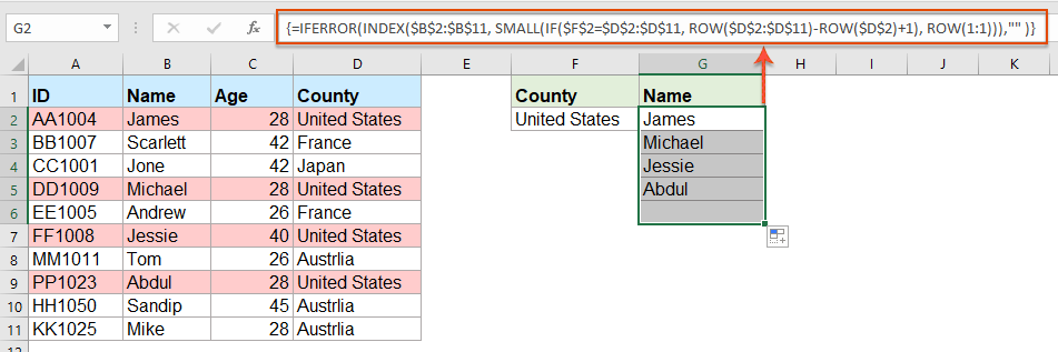
1. Kopiera eller skriv in formeln nedan i en tom cell där du vill hitta resultatet:

=INDEX($B$2:$B$11, SMALL(IF(COUNTIF($F$2, $C$2:$C$11)*COUNTIF($G$2, $D$2:$D$11), ROW($A$2:$D$11)-MIN(ROW($A$2:$D$11))+1), ROW(A1)), COLUMN(A1))

Anmärkningar: I ovanstående formel, B2: B11 är den kolumn som matchande värde returneras från; F2, C2: C11 är det första villkoret och kolumndata som innehåller det första villkoret; G2, D2: D11 är det andra villkoret och kolumndata som innehåller detta villkor, ändra dem till ditt behov.

2. Tryck sedan på Ctrl + Skift + Enter för att få det första matchningsresultatet och välj sedan den första formelcellen och dra påfyllningshanteringen ner till cellerna tills felvärdet visas. Nu returneras alla matchande värden som visas nedan:

tips: Om du bara behöver returnera alla matchande värden baserat på ett villkor, använd nedanstående matrisformel:

=IFERROR(INDEX($B$2:$B$11, SMALL(IF($F$2=$D$2:$D$11, ROW($D$2:$D$11)-ROW($D$2)+1), ROW(1:1))),"" )


Fler relativa artiklar:

  • Returnera flera sökvärden i en kommaseparerad cell
  • I Excel kan vi använda VLOOKUP-funktionen för att returnera det första matchade värdet från en tabellceller, men ibland måste vi extrahera alla matchande värden och sedan separeras med en specifik avgränsare, som komma, bindestreck, etc ... i en enda cell som följande skärmdump visas. Hur kunde vi få och returnera flera uppslagsvärden i en kommaseparerad cell i Excel?
  • Vlookup och returnera flera matchande värden på en gång i Google Sheet
  • Den normala Vlookup-funktionen i Google-ark kan hjälpa dig att hitta och returnera det första matchande värdet baserat på en viss data. Men ibland kan du behöva slå upp och returnera alla matchande värden enligt följande skärmdump. Har du några bra och enkla sätt att lösa denna uppgift i Google-ark?
  • Vlookup och returnera flera värden från rullgardinslistan
  • I Excel, hur kan du söka efter och returnera flera motsvarande värden från en rullgardinslista, vilket innebär att när du väljer ett objekt från listrutan, visas alla dess relativa värden på en gång som följande skärmdump visas. Den här artikeln presenterar jag lösningen steg för steg.
  • Vlookup och returnera flera värden vertikalt i Excel
  • Normalt kan du använda Vlookup-funktionen för att få det första motsvarande värdet, men ibland vill du returnera alla matchande poster baserat på ett specifikt kriterium. Den här artikeln kommer jag att prata om hur man slår på och returnerar alla matchande värden vertikalt, horisontellt eller i en enda cell.
  • Vlookup och returnera matchande data mellan två värden i Excel
  • I Excel kan vi använda den normala Vlookup-funktionen för att få motsvarande värde baserat på en viss data. Men ibland vill vi söka efter och returnera matchningsvärdet mellan två värden som följande skärmdump visas, hur kan du hantera den här uppgiften i Excel?


  • Super Formula Bar (enkelt redigera flera rader med text och formel); Läslayout (enkelt läsa och redigera ett stort antal celler); Klistra in i filtrerat intervall...
  • Sammanfoga celler / rader / kolumner och förvaring av data; Delat cellinnehåll; Kombinera duplicerade rader och summa / genomsnitt... Förhindra duplicerade celler; Jämför intervall...
  • Välj Duplicera eller Unikt Rader; Välj tomma rader (alla celler är tomma); Super Find och Fuzzy Find i många arbetsböcker; Slumpmässigt val ...
  • Exakt kopia Flera celler utan att ändra formelreferens; Skapa referenser automatiskt till flera ark; Sätt in kulor, Kryssrutor och mer ...
  • Favorit och sätt snabbt in formler, Intervall, diagram och bilder; Kryptera celler med lösenord; Skapa e-postlista och skicka e-post ...
  • Extrahera text, Lägg till text, ta bort efter position, Ta bort mellanslag; Skapa och skriva ut personsökningstalsatser; Konvertera mellan celler innehåll och kommentarer...
  • Superfilter (spara och tillämpa filterscheman på andra ark); Avancerad sortering efter månad / vecka / dag, frekvens och mer; Specialfilter av fet, kursiv ...
  • Kombinera arbetsböcker och arbetsblad; Sammanfoga tabeller baserat på nyckelkolumner; Dela data i flera ark; Batchkonvertera xls, xlsx och PDF...
  • Gruppering av pivottabell efter veckonummer, veckodagen och mer ... Visa olåsta, låsta celler av olika färger; Markera celler som har formel / namn...
kte-flik 201905
  • Aktivera flikredigering och läsning i Word, Excel, PowerPoint, Publisher, Access, Visio och Project.
  • Öppna och skapa flera dokument i nya flikar i samma fönster, snarare än i nya fönster.
  • Ökar din produktivitet med 50 % och minskar hundratals musklick för dig varje dag!
officetab botten


Comments (25)
No ratings yet. Be the first to rate!
This comment was minimized by the moderator on the site
Hi, if there are duplicate values (e.g. two adams), how do i make sure that it only returns 1 adam and not 2?
This comment was minimized by the moderator on the site
Hello, Bobby,
To extract only unique matching values, you should apply the below formula:
After pasting the formula, please press Ctrl + Shift + Enter keys together to get the correct result.
=IFERROR(INDEX($B$2:$B$5, MATCH(0, COUNTIF(H1:$H$1, $B$2:$B$5)+IF($D$2:$D$5<>$G$2, 1, 0)+IF($C$2:$C$5<>$F$2, 1, 0), 0)), "")

Please have a try, hope it can help you!
This comment was minimized by the moderator on the site
Hi,

Thanks for posting these examples.
I'm trying to implement this in my own sheet, but don't get it to work (maybe because I'm using an europe version of excel)?

I want to get the dates of the days that I had my shifts or that I have worked 'some' (>0) hours for a client.

So in I3 is the name and in J3 the month. K3 and L3 are the shifts (1 is worked) and hours (don't know how to set this, should be more than zero)

My expected results are in:
Shifts: I7 and I8
hours: J7

So I worked more than 0 hours for 'person 2' in oktober on 3-10-2022
had shifts for person 2 on '10-10-2022' and 28-10-2022

When I add '=INDEX($B$2:$B$11, SMALL(IF(COUNTIF($F$2, $C$2:$C$11)*COUNTIF($G$2, $D$2:$D$11), ROW($A$2:$D$11)-MIN(ROW($A$2:$D$11))+1), ROW(A1)), COLUMN(A1))' in my excel sheet, it doesn't allow the comma between the different parts of the formula.
So I need to change them to ';'.
But when I try it it always says: '#NAME?'

So can someone help me with this?

Kind regards,

Bas
[img]https://drive.google.com/file/d/1iIPQKuj_PNhqWyWlwJ4IQTqGNEd6B9Hw/view?usp=share_link[/img]
This comment was minimized by the moderator on the site
Hi,

First, thank you for sharing!

Can you please provide a solution to the case below:

I have 3 columns (A: Containing reference information, B: Containing information to be searched, C: Search result)

Image url is provided below

https://ibb.co/VHCd09K

Column A-------------------------Column B------------Column C
File Name-------------------------Name----------------File Name, Document Name, Element Name, Name
Changed Element-----------------Element--------------Changed Element, Element Name, Element ID
Column Location
Document Name
Element Name
Name
Category
Warranty
Slope
Element ID

What I need is to search in column A for any partial match with cell B2 (Name) or B3 (Element) and get the result in one cell,

Thank you, Behzad
This comment was minimized by the moderator on the site
Hello, Behzad
Maybe the below User Defined Function can help you.
Public Function ConcatPartLookUp(rngInput As Range, rngSource As Range, Optional strDelimiter As String, Optional blCaseSensitive)
Dim rng As Range
If strDelimiter = "" Then strDelimiter = ","
If IsMissing(blCaseSensitive) Then
    blCaseSensitive = False
Else
    blCaseSensitive = True
End If
For Each rng In rngSource
    If blCaseSensitive Then
        If InStr(1, rng.Value, rngInput.Value, vbBinaryCompare) > 0 Then ConcatPartLookUp = ConcatPartLookUp & strDelimiter & rng.Value
    Else
        If InStr(1, rng.Value, rngInput.Value, vbTextCompare) > 0 Then ConcatPartLookUp = ConcatPartLookUp & strDelimiter & rng.Value
    End If
Next
If Len(ConcatPartLookUp) > 0 Then ConcatPartLookUp = Mid(ConcatPartLookUp, 2, Len(ConcatPartLookUp))
End Function


After copying and pasting this code, and then use this formula:=ConcatPartLookUp(B2,$A$2:$A$8) to get the result you need.
Please have a try, hope it can help you!
This comment was minimized by the moderator on the site
Heyi, thank you for the formula. It worked for "fixed" values / text as criterias. However, one of the criterias i'm trying to use is a condition (values <>0 ), but does not work the described formula. Do you guys know what should i change to adapt the formula so I can have a condition as one of the criterias, please?

Best,

João
This comment was minimized by the moderator on the site
Hello, Marcus
To solve your problem, please view this article:
https://www.extendoffice.com/documents/excel/6393-excel-vlookup-function.html#b3-2
There are some detailed explanations of this task. You just need to change the criteira to your own.
Thank you!
This comment was minimized by the moderator on the site
Hi,

if in cell H1 i write "Name" and wanted to link that with the formula, how would that work?
Then I could write "ID" in cell H1 and would automatically get as a result: AA1004; DD1009; PP1023 (for the first formula)

Thank you in advance!
This comment was minimized by the moderator on the site
Hello, Marie
Sorry, i can't get the point of your first problem, could you explain your problem more clearly and detailedly? Or you can insert a screenshot here to describe your problem.
As for the second question, you just need to change the cell reference as this:
=INDEX($A$2:$A$11, SMALL(IF(COUNTIF($F$2, $C$2:$C$11)*COUNTIF($G$2, $D$2:$D$11), ROW($A$2:$D$11)-MIN(ROW($A$2:$D$11))+1), ROW(A1)), COLUMN(A1))

Remeber to press Ctrl + Shift + Enter keys together.
Please try, hope it can help you!
This comment was minimized by the moderator on the site
Hello,
what would be needed to expand the first formula in the following case:
Some IDs are Blank (e.g. cell A5 is blank) and I would like an additional condition outputting lines only when the IDs are not blank. (So the output should then be James and Abdul.
Thanks!
This comment was minimized by the moderator on the site
Hello, Jo,
To solve your problem, please apply the below formula:
=INDEX($B$2:$B$11, SMALL(IF(COUNTIF($F$2, $C$2:$C$11)*COUNTIF($G$2, $D$2:$D$11)*($A$2:$A$11<>0), ROW($A$2:$D$11)-MIN(ROW($A$2:$D$11))+1), ROW(A1)), COLUMN(A1))

Please have a ry, hope it can help you!
This comment was minimized by the moderator on the site
hello,
ive tried using the formula and it either generates a value of 0 or the image attached
This comment was minimized by the moderator on the site
Hello, Milku
Your screenshot showed WPS software of MAC version, so I am not sure whether our formula is available.
I uploaded an Excel file to here, you can try to see if it can calculate correctly in you environment.
Thank you!
This comment was minimized by the moderator on the site
When I use the second formula and drag down, nothing appears. The formula result (fx) says it should be returning something but it is blank. How do I correct this?
This comment was minimized by the moderator on the site
Hello Alysia,

Glad to help. I tried the second formula in the article and drag the formula down, the rest of results were returned. I think there may be two reasons for your problem. First, maybe you forget to press Ctrl + Shift + Enter keys to enter the formula. Second, the matching result is only one, so no other results are not returned. Please have a check.

Sincerely,
Mandy
This comment was minimized by the moderator on the site
Hi,

I was wondering if it at all possible to enter a 2nd criteria but from the same range as the 1st criteria,

For example with the used example above i would like to search for the names of people from both America and France So cell F3 would have France, Scarlett & Andrew would also populate in the list in Column G

Thank you for assistance in advance.
This comment was minimized by the moderator on the site
Hello Nick,

Glad to help. If you want to get the names of people from both America and France, I advise you to use our formula twice to get the result. Please see the screenshot, In F2 and G2 are values "United States" and "France". Apply formula =IFERROR(INDEX($B$2:$B$11, SMALL(IF($F$2=$D$2:$D$11, ROW($D$2:$D$11)-ROW($D$2)+1), ROW(1:1))),"" ) to get the results for America. And apply formula =IFERROR(INDEX($B$2:$B$11, SMALL(IF($G$2=$D$2:$D$11, ROW($D$2:$D$11)-ROW($D$2)+1), ROW(1:1))),"" ) to get the results for France. It's simple. Please have a try.

Sincerely,
Mandy
This comment was minimized by the moderator on the site
In the first example, what change to the formula would be needed to return everyone who was less than 28 years old?
There are no comments posted here yet
Load More
Please leave your comments in English
Posting as Guest
×
Rate this post:
0   Characters
Suggested Locations