Hoppa till huvudinnehåll

Hur ändrar jag bakgrunds- eller teckensnittsfärg baserat på cellvärde i Excel?

När du hanterar enorma data i Excel kanske du vill välja något värde och markera dem med specifik bakgrunds- eller teckensnittsfärg. Den här artikeln talar om hur du snabbt ändrar bakgrunds- eller teckensnittsfärgen baserat på cellvärden i Excel.


Metod 1: Ändra bakgrunds- eller teckensnittsfärg baserat på cellvärde dynamiskt med villkorlig formatering


Smakämnen Villkorlig formatering funktionen kan hjälpa dig att markera värden större än x, mindre än y eller mellan x och y.

Om du antar att du har en rad data, och nu måste du färga värdena mellan 80 och 100, gör med följande steg:

1. Välj det cellområde som du vill markera vissa celler och klicka sedan på Hem > Villkorlig formatering > Ny regel, se skärmdump:

doc markera med värde 1

2. I Ny formateringsregel dialogrutan väljer du Formatera endast celler som innehåller objekt i Välj en regeltyp rutan och i Formatera endast celler med avsnittet, ange villkoren du behöver:

  • Välj den i den första rullgardinsmenyn Cellvärde;
  • Välj kriterierna i den andra rullgardinsmenyn:mellan;
  • I den tredje och fjärde rutan anger du filtervillkoren, till exempel 80, 100.

doc markera med värde 2

3. Klicka sedan bildad knappen, i Formatera celler dialogrutan, ställ in bakgrunds- eller teckensnittsfärgen så här:

Ändra bakgrundsfärgen efter cellvärde: Ändra teckensnittsfärgen efter cellvärde
Klicka Fyll och välj sedan en bakgrundsfärg som du gillar Klicka Font och välj den teckensnittsfärg du behöver.
doc markera med värde 3 doc markera med värde 4

4. Efter att ha valt bakgrunds- eller teckensnittsfärg, klicka OK > OK för att stänga dialogerna, och nu ändras de specifika cellerna med ett värde mellan 80 och 100 till det som bakgrunden eller teckensnittsfärgen i valet. Se skärmdump:

Markera specifika celler med bakgrundsfärg: Markera specifika celler med teckensnittsfärg:
doc markera med värde 5 doc markera med värde 6

Anmärkningar: Den Villkorlig formatering är en dynamisk funktion kommer cellfärgen att ändras när data ändras.


Metod 2: Ändra bakgrunds- eller teckensnittsfärg baserat på cellvärde statiskt med Sök-funktionen


Ibland måste du använda en specifik fyllnings- eller teckensnittsfärg baserat på cellvärde och se till att fyllningen eller teckensnittsfärgen inte ändras när cellvärdet ändras. I det här fallet kan du använda hitta funktion för att hitta alla specifika cellvärden och sedan ändra bakgrunds- eller teckensnittsfärgen efter dina behov.

Du vill till exempel ändra bakgrunds- eller teckensnittsfärgen om cellvärdet innehåller "Excel" -text, gör så här:

1. Välj det dataområde du vill använda och klicka sedan på Hem > Hitta och välj > hitta, se skärmdump:

doc markera med värde 7

2. I Sök och ersätt under dialogrutan hitta fliken, ange det värde som du vill hitta i Hitta det textruta, se skärmdump:

doc markera med värde 8

tips: Om du behöver hitta värdena med skiftlägeskänslig eller matcha hela cellinnehållet, klicka på Tillbehör för att få avancerade sökalternativ, till exempel "match Case"Och"Matcha hela cellinnehållet"som du behöver.

3. Och klicka sedan på Hitta alla , klicka på valfritt objekt i sökresultatrutan och tryck sedan på Ctrl + A för att välja alla hittade objekt, se skärmdump:

doc markera med värde 9

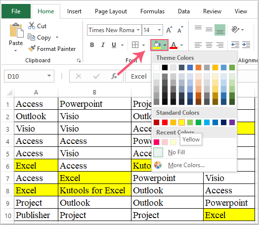
4. Äntligen klickar du på Stänga för att stänga denna dialog. Nu kan du fylla en bakgrunds- eller teckensnittsfärg för dessa valda värden, se skärmdump:

Tillämpa bakgrundsfärgen för de valda cellerna: Använd teckensnittsfärgen för de valda cellerna:
doc markera med värde 10 doc markera med värde 11

Metod 3: Ändra bakgrunds- eller teckensnittsfärg baserat på cellvärde statiskt med Kutools för Excel


Kutools för ExcelÄr Superfynd funktionen stöder många villkor för att hitta värden, textsträngar, datum, formler, formaterade celler och så vidare. När du har hittat och valt de matchade cellerna kan du ändra bakgrunds- eller teckensnittsfärgen till önskad.

När du har installerat Kutools för Excel, gör så här:

1. Välj det dataområde som du vill hitta och klicka sedan på Kutools > Superfynd, se skärmdump:

doc markera med värde 12

2. I Superfynd i rutan, gör följande:

  • (1.) Klicka först på Värden alternativikon;
  • (2.) Välj sökområdet från Inom rullgardinsmeny, i det här fallet väljer jag Urval;
  • (3.) Från Typ rullgardinslista, välj de kriterier som du vill använda;
  • (4.) Klicka sedan på hitta knapp för att lista alla motsvarande resultat i listrutan;
  • (5.) Klicka äntligen på Välja för att välja celler.

doc markera med värde 13

3. Och sedan har alla celler som matchar kriterierna valts på en gång, se skärmdump:

doc markera med värde 14

4. Och nu kan du ändra bakgrundsfärgen eller teckensnittsfärgen för de valda cellerna efter behov.


Upptagen arbete på helgen, Använd Kutools för Excel,
ger dig en avkopplande och glad helg!

På helgen klagar barnen för att leka, men det finns för mycket arbete som omger dig för att få tid att följa med familjen. Solen, stranden och havet så långt borta? Kutools för Excel hjälper dig att lösa Excel-pussel, spara arbetstid.

pic strand
  •  Få en befordran och öka lönen är inte långt borta;
  •  Innehåller avancerade funktioner, lös applikationsscenarier, vissa funktioner sparar till och med 99 % arbetstid;
  •  Bli en expert på 3 minuter och få erkännande från dina kollegor eller vänner;
  •  Behöver inte längre söka lösningar från Google, säga adjö till smärtsamma formler och VBA-koder;
  •  Alla upprepade operationer kan slutföras med bara flera klick, frigör dina trötta händer;
  •  Endast $ 39 men värt än andras $ 4000 Excel-handledning;
  •  Bli vald av 110,000 300 eliter och XNUMX+ välkända företag;
  •  30-dagars gratis provperiod och fulla pengarna tillbaka inom 60 dagar utan någon anledning;
  •  Ändra ditt sätt att arbeta och ändra sedan din livsstil!
 

Comments (79)
No ratings yet. Be the first to rate!
This comment was minimized by the moderator on the site
Good Day,

I have a schedule with different course modules that can be placed in different order ( 1 is metal, 2 is machining, 3 is refinishing, etc.) depending on course director preferences and staff availability.

What I am trying to do to wrap up the spreadsheet is color code the modules across the months based on their order in the overall course. So if Metal is first and is 35 days long, the first 35 days are background colored blue, but if machining is first and is 20 days long, then the first 20 days are purple.

How can you do and if statement that refers to a separate cell for the initial number of days, AND color the cells based on the range between 1 and 20 or 35 or whatever?

Can I do a conditional formatting If statement with a range between numbers?

This would have to be applied to all the modules (therefor multiple conditional formatting formulas) to account for any module being in any place in the order.
That is the issue I have. Please offer any suggestions. Note that I have built the spreadsheet without VBA. (I've never had the opportunity to learn it)
This comment was minimized by the moderator on the site
Can I give colour for a row of values with respect to previous value for a whole row.
Eg

23

45

32

56

can I give red for 23 and green for 45 and again red for 32 as it is less than the previous value and green for 56 as it is more than 32.
This comment was minimized by the moderator on the site
I do get to change a cell colour according to the text or letter in fill in the cell e.g.-H=YELLOW,E=GREEN
This comment was minimized by the moderator on the site
Hello, VANESSA,
For solving your problem, please apply the Conditional Formatting feature, in the New Formatting Rule dialog box, choose the conditions as following screenshot shown:
This comment was minimized by the moderator on the site
how do i change the colour of cell depending on what is in that cell IE. Y=green N=red.

thats how i need it if it has Y riten in the cell it turns green?
This comment was minimized by the moderator on the site
Hello, Leon,
To highlight the cells based on the cell value, you should apply the Conditional Formatting feature, go to the New Formatting Rule dialog box, and then do as the following screenshot shown to highlight the cells which are Y located as green:

Do with the same way to format the cells N as red color.

Please try it, hope it can help you!
This comment was minimized by the moderator on the site
Trying to get a cell to highlight if its above a certain number, the problem is that the cell includes the number and a date. Is there a way i can get it to just look at the number? The cell will include a number+date.....1400(7/2/2018). I need the formulate just to look at the 1400 and not the date.
any ideas?
thanks
Z
This comment was minimized by the moderator on the site
Sir, I have value in cell A10, in A12. Now I entered a simple formula in A15 subtracting these (A10-A12). I want background color of result cell (A15) in green if A10 is large (means result in positive number) and background color in red if A12 is large ( result in negative number). Please provide solution
This comment was minimized by the moderator on the site
Hello,
You can select the formula cells, and then apply the Conditional Formatting > Greater than (0)-format it green, and then Less Than (0)-format it red, see screenshot:

Please try it, hope it can help you, thank you!
This comment was minimized by the moderator on the site
If I have a date in a cell, how do I make it change to orange when it is within 30 days of coming due, yellow when it is within 15 days of coming due and red when it exceeds the date (past due)
This comment was minimized by the moderator on the site
I thought this color of cells by value was going to be a real pain. It could not have been explained more easily and clearly. Thanks. It took no less than 1-2 minutes to understand what to do.
This comment was minimized by the moderator on the site
HI, I want if i change any value or number in any cell then that cell text color should get change for e.g. if number in any cell is 100 and I have to change it as 98 then that cell text 98 should change into red color. Is it possible in Excel?? Do clarify please
This comment was minimized by the moderator on the site
So I am creating a excel spreadsheet for fire department reports. What I am looking for is it to calculate the days a report is overdue, unless it has been completed: Column A Column B Column C Column D Column E Column F Incident # Incident Date Todays Date Completed Date Days Overdue Todays Date I want column B subtracting Column C to calculate in column E unless Column D is complete. I hope this makes sense. I want to use the conditional formatting to show me in colors how long a report is overdue (with the 3 color scale). I have the formula for the number of days it is overdue to have a correct value and color scale, but I want it to remain green when the report has been completed.
There are no comments posted here yet
Load More
Please leave your comments in English
Posting as Guest
×
Rate this post:
0   Characters
Suggested Locations