Hoppa till huvudinnehåll

Hur döljer jag noll dataetiketter i diagram i Excel?

Författare: Sun Senast ändrad: 2014-09-18

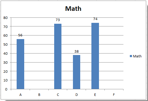
Ibland kan du lägga till dataetiketter i diagrammet för att göra datavärdet tydligare och direkt i Excel. Men i vissa fall finns det noll dataetiketter i diagrammet, och du kanske vill dölja dessa nolldatatiketter. Här kommer jag att berätta ett snabbt sätt att dölja nolldatatiketterna i Excel på en gång.

Dölj noll dataetiketter i diagrammet


pil blå höger bubbla Dölj noll dataetiketter i diagrammet

Gör så här om du vill dölja noll dataetiketter i diagrammet:

1. Högerklicka på en av datatiketterna och välj Formatera datatiketter från snabbmenyn. Se skärmdump:

doc-hide-zero-data-label-1

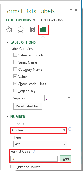
2. I Formatera datatiketter Klicka på Antal i vänster ruta och välj sedan Anpassad från kategorin listrutan och skriv # "" i Formatkod textruta och klicka Lägg till knappen för att lägga till den till Typ listruta. Se skärmdump:

doc-hide-zero-data-label-2

3. klick Stänga för att stänga dialogrutan. Då kan du se alla noll dataetiketter är dolda.

doc-hide-zero-data-label-3

Tips: Om du vill visa nolldatamärkarna, gå tillbaka till dialogrutan Formatera datatiketter och klicka Antal > Custom, och välj #, ## 0; - #, ## 0 i Typ listrutan.

Anmärkningar: I Excel 2013 kan du högerklicka på valfri datatikett och välja Formatera datatiketter att öppna Formatera datatiketter ruta; Klicka sedan Antal att utöka sitt alternativ; klicka sedan på Kategori och välj Custom från listrutan och skriv # "" i Formatkod textrutan och klicka på Lägg till knapp.

doc-hide-zero-data-label-4


Relativa artiklar:

Bästa kontorsproduktivitetsverktyg

🤖 Kutools AI Aide: Revolutionera dataanalys baserat på: Intelligent utförande   |  Generera kod  |  Skapa anpassade formler  |  Analysera data och generera diagram  |  Anropa Kutools funktioner.
Populära funktioner: Hitta, markera eller identifiera dubbletter   |  Ta bort tomma rader   |  Kombinera kolumner eller celler utan att förlora data   |   Rund utan formel ...
Superuppslag: Flera kriterier VLookup    VLookup med flera värden  |   VSök över flera ark   |   Fuzzy Lookup ....
Avancerad rullgardinslista: Skapa snabbt en rullgardinslista   |  Beroende rullgardinslista   |  Flervals-rullgardinslista ....
Kolumnhanterare: Lägg till ett specifikt antal kolumner  |  Flytta kolumner  |  Växla synlighetsstatus för dolda kolumner  |  Jämför intervall och kolumner ...
Utvalda funktioner: Rutnätsfokus   |  Designvy   |   Stor formelbar    Arbetsbok & Bladhanterare   |  Resursbibliotek (Automatisk text)   |  Datumväljare   |  Kombinera arbetsblad   |  Kryptera/Dekryptera celler    Skicka e-postmeddelanden efter lista   |  Superfilter   |   Specialfilter (filtrera fet/kursiv/genomstruken...) ...
Topp 15 verktygssatser12 text verktyg (lägga till text, Ta bort tecken, ...)   |   50+ Diagram Typer (Gantt Chart, ...)   |   40+ Praktiskt Formler (Beräkna ålder baserat på födelsedag, ...)   |   19 Införande verktyg (Infoga QR-kod, Infoga bild från sökväg, ...)   |   12 Konvertering verktyg (Siffror till ord, Valutaväxling, ...)   |   7 Slå ihop och dela verktyg (Avancerade kombinera rader, Dela celler, ...)   |   ... och mer

Uppgradera dina Excel-färdigheter med Kutools för Excel och upplev effektivitet som aldrig förr. Kutools för Excel erbjuder över 300 avancerade funktioner för att öka produktiviteten och spara tid.  Klicka här för att få den funktion du behöver mest...

Beskrivning


Fliken Office ger ett flikgränssnitt till Office och gör ditt arbete mycket enklare

  • Aktivera flikredigering och läsning i Word, Excel, PowerPoint, Publisher, Access, Visio och Project.
  • Öppna och skapa flera dokument i nya flikar i samma fönster, snarare än i nya fönster.
  • Ökar din produktivitet med 50 % och minskar hundratals musklick för dig varje dag!
Comments (15)
No ratings yet. Be the first to rate!
This comment was minimized by the moderator on the site
Muito obrigado!
This comment was minimized by the moderator on the site
Depending on your data set, you could use a helper column. The formula could use rounddown or IF(cell<1,0,cell). This way your slicers stay intact and your pie chart uses the new column.
This comment was minimized by the moderator on the site
I have a pivot chart (pie chart) where I need to remove the labels for any slice of the pie with a value under 1%. Right now, these are displayed as 0% (no decimal places). I am also using slicers to analyse the data by month, department and person. I am trying to get the chart to hide any labels where the value is less than 1%, but this will change when I change the variables in the slicers. I have fallen down a rabbit-hole here trying to figure this out.
This comment was minimized by the moderator on the site
The Microsoft way of doing it (though not found on ana MS help page) is to click File>Options>Advanced, scroll down to 'Display options for this worksheet', and uncheck / untick 'Show a zero in cells that have a zero value'. All the zeros disappear.

I seem to have found a way to remove the axis name and space on a graph or chart for zero values: Highlight the whole table, click Home>Sort and filter>Filter, Click on the header of the column with the blank zero values, and uncheck / untick 'Blanks'.
This comment was minimized by the moderator on the site
Thanks that really works well for me.
This comment was minimized by the moderator on the site
tnx, it works
This comment was minimized by the moderator on the site
How can I hide Zero Data Labels when it is percentage (for example 0,00%, I do not want that label to be shown)?
This comment was minimized by the moderator on the site
<span style="letter-spacing: 0.2px; color: inherit; font-family: inherit; font-style: inherit; font-variant-ligatures: inherit; font-variant-caps: inherit; font-weight: inherit;">0.0%;-0.0%;""    </span>
This comment was minimized by the moderator on the site
Hi
Thank you for sharing the solution above. It was really great help. However, after hiding zero values, I am having difficulties with hiding their labels. Can you please give a solution for that problem, too? Thank in advance for your help.
This comment was minimized by the moderator on the site
Found this solution absolutely useful. Thanks a ton.
This comment was minimized by the moderator on the site
Great solution! Can this be done retaining decimal points on the numbers that do appear?
This comment was minimized by the moderator on the site
Kelcey, use: #,##"";-#,##""; When using the second semicolon, you define what happens in case of zero. So, if you don't define anything, the value stays blank.
This comment was minimized by the moderator on the site
I use 0.0;;; and it also does the trick, in terms of retaining decimal places. You'd just adjust to the # of sig figs you want to keep. You have to assign the custom value to each data label series, but it keeps that format each time you refresh the data.
There are no comments posted here yet
Load More
Please leave your comments in English
Posting as Guest
×
Rate this post:
0   Characters
Suggested Locations