Hoppa till huvudinnehåll

Hur skapar jag en beroende rullgardinslista i Google-ark?

Författare: Xiaoyang Senast ändrad: 2020-11-25

Att infoga en normal rullgardinslista i Google-ark kan vara ett enkelt jobb för dig, men ibland kan du behöva infoga en beroende rullgardinsmeny, vilket betyder den andra rullgardinsmenyn beroende på valet av den första rullgardinsmenyn. Hur kan du hantera den här uppgiften i Google-ark?

Skapa en beroende rullgardinslista i Google-ark


Skapa en beroende rullgardinslista i Google-ark

Följande steg kan hjälpa dig att infoga en beroende rullgardinslista, gör så här:

1. Först bör du infoga den grundläggande rullgardinsmenyn, välj en cell där du vill placera den första rullgardinsmenyn och klicka sedan Data > Datavalidering, se skärmdump:

2. I poppade ut Datavalidering dialogrutan väljer du Lista från ett intervall från rullgardinsmenyn bredvid Kriterier och klicka sedan på för att välja cellvärdena som du vill skapa den första rullgardinsmenyn baserat på, se skärmdump:

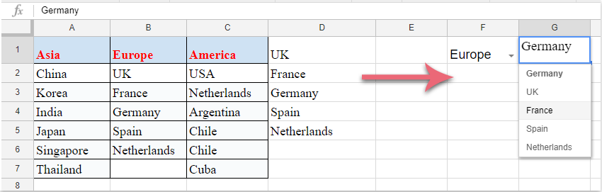
3. Klicka sedan Save knappen har den första rullgardinsmenyn skapats. Välj ett objekt i den skapade rullgardinsmenyn och ange sedan denna formel: =arrayformula(if(F1=A1,A2:A7,if(F1=B1,B2:B6,if(F1=C1,C2:C7,"")))) in i en tom cell som ligger intill datakolumnerna och tryck sedan på ange nyckel, alla matchande värden baserade på det första listrutan har visats på en gång, se skärmdump:

Anmärkningar: I ovanstående formel: F1 är den första rullgardinsmenyn, A1, B1 och C1 är artiklarna i den första rullgardinsmenyn, A2: A7, B2: B6 och C2: C7 är cellvärdena som den andra rullgardinsmenyn baseras på. Du kan ändra dem till dina egna.

4. Och sedan kan du skapa den andra beroende rullgardinsmenyn, klicka på en cell där du vill placera den andra rullgardinsmenyn och klicka sedan på Data > Datavalidering för att gå till Datavalidering dialogrutan, välj Lista från ett intervall från rullgardinsmenyn bredvid Kriterier och klicka på knappen för att välja formelcellerna som är matchande resultat för det första rullgardinsobjektet, se skärmdump:

5. Klicka äntligen på knappen Spara, och den andra beroende rullgardinsmenyn har skapats framgångsrikt som följande skärmdump visas:

Bästa kontorsproduktivitetsverktyg

🤖 Kutools AI Aide: Revolutionera dataanalys baserat på: Intelligent utförande   |  Generera kod  |  Skapa anpassade formler  |  Analysera data och generera diagram  |  Anropa Kutools funktioner.
Populära funktioner: Hitta, markera eller identifiera dubbletter   |  Ta bort tomma rader   |  Kombinera kolumner eller celler utan att förlora data   |   Rund utan formel ...
Superuppslag: Flera kriterier VLookup    VLookup med flera värden  |   VSök över flera ark   |   Fuzzy Lookup ....
Avancerad rullgardinslista: Skapa snabbt en rullgardinslista   |  Beroende rullgardinslista   |  Flervals-rullgardinslista ....
Kolumnhanterare: Lägg till ett specifikt antal kolumner  |  Flytta kolumner  |  Växla synlighetsstatus för dolda kolumner  |  Jämför intervall och kolumner ...
Utvalda funktioner: Rutnätsfokus   |  Designvy   |   Stor formelbar    Arbetsbok & Bladhanterare   |  Resursbibliotek (Automatisk text)   |  Datumväljare   |  Kombinera arbetsblad   |  Kryptera/Dekryptera celler    Skicka e-postmeddelanden efter lista   |  Superfilter   |   Specialfilter (filtrera fet/kursiv/genomstruken...) ...
Topp 15 verktygssatser12 text verktyg (lägga till text, Ta bort tecken, ...)   |   50+ Diagram Typer (Gantt Chart, ...)   |   40+ Praktiskt Formler (Beräkna ålder baserat på födelsedag, ...)   |   19 Införande verktyg (Infoga QR-kod, Infoga bild från sökväg, ...)   |   12 Konvertering verktyg (Siffror till ord, Valutaväxling, ...)   |   7 Slå ihop och dela verktyg (Avancerade kombinera rader, Dela celler, ...)   |   ... och mer

Uppgradera dina Excel-färdigheter med Kutools för Excel och upplev effektivitet som aldrig förr. Kutools för Excel erbjuder över 300 avancerade funktioner för att öka produktiviteten och spara tid.  Klicka här för att få den funktion du behöver mest...

Beskrivning


Fliken Office ger ett flikgränssnitt till Office och gör ditt arbete mycket enklare

  • Aktivera flikredigering och läsning i Word, Excel, PowerPoint, Publisher, Access, Visio och Project.
  • Öppna och skapa flera dokument i nya flikar i samma fönster, snarare än i nya fönster.
  • Ökar din produktivitet med 50 % och minskar hundratals musklick för dig varje dag!
Comments (18)
No ratings yet. Be the first to rate!
This comment was minimized by the moderator on the site
Hi there. Its been working but for it only appears that only one cell can be formulated.I need help 
For example: in Cell A1, it shows dependent dropdown, but when in cell a2 it does not work.
Thas what help that i need, From A:A, They have all different selection from the dropdown list. Thanks.
This comment was minimized by the moderator on the site
Would it been possible to create pull down menu based of formula?
I use formula "=SUMIFS(Items!$I:$I,Items!$A:$A,K$1,Items!$D:$D,$D2)" (=for example 150) to find the qty on pallet based on item and container size.
So I wanted to create pull down menu like qty 1 pallet, qty 2 pallets, qty 3 pallets,.....
Then user will always order qty of full pallets like 150, 2 x 150, 3 x150, up to 21 x 150.
This comment was minimized by the moderator on the site
Hi, I already created a drop down list like this one, what I'd like to know is how i can, when clicking on one option from that list, restrict what appears as options on another cell. For example, in one cell i can choose between laparoscopy and orthopaedics. If I choose orthopaedics then, the other cell which has a list of doctors, should only show the doctors for orthopedy and not all of them. Does anyone know how to do this?
This comment was minimized by the moderator on the site
Hii Sir,
I Want to Create A Dependent Drop Down List Like
- State(A1):- District(B1):- Taluka(C1) :- Then Information(D1) ,
So I need your Help .
Tell How do you do this Type of Dependent Drop down List in Excel or Google Sheet
This comment was minimized by the moderator on the site
Hi, Shelate,
Maybe the below article can solve your problem, please view it:
https://www.extendoffice.com/documents/excel/5852-excel-multiple-level-drop-down-list.html

Please try, hope it can help you!
This comment was minimized by the moderator on the site
Now is needed to use: =arrayformula(if(F1=A1;A2:A7;if(F1=B1;B2:B6;if(F1=C1;C2:C7;""))))
This comment was minimized by the moderator on the site
Thank you soooo much!
This comment was minimized by the moderator on the site
Hi,
I was wondering if anyone could advise me with this? I've followed the above steps but on step 3 rather than getting:
"...all the matching values based on the first drop down list item have been displayed at once," I am just seeing one value (the top one from the drop down list).
My cells are placed slightly differently and the first drop down is filled from another sheet (from anywhere int eh column excluding the top row) so my formula is:

=arrayformula(if(VLE!D2:D=B11,B12,if(VLE!D2:D=C11,C12:C14,if(VLE!D2:D=D11,D12:D14,if(VLE!D2:D=E11,E12:E16,if(VLE!D2:D=F11,F12:F16,""))))))

It is correctly displaying the top drop down option for each of (using cell numbers from the step 3 example on this page) A1, B1, and C1 so, again using this page's example, if I select Asia form the F1 drop down, I would get China, but nothing further


Any suggestions?

Many thanks! Nick
This comment was minimized by the moderator on the site
If the first drop own is on sheet 1 A1, will this work were I want the second drop down as sheet 1 A2, but to have its data range on a separate sheet?
This comment was minimized by the moderator on the site
Ich bekomm immer die Meldung "Fehler beim Parsen der Formel" wenn ich =arrayformula(if(F1=A1,A2:A7,if(F1=B1,B2:B6,if(F1=C1,C2:C7,"")))) eingebe. Was ist der "Weiter-Schlüsel"? Reicht es nicht wie bei Excel die Formel einzugeben?
This comment was minimized by the moderator on the site
Ersetzen Sie den , zu ;
es hat für mich funktioniert
This comment was minimized by the moderator on the site
This is the best explanation I have found, so thank you for that!

In my situation, I am working with over 200 rows with more being continuously added. Is there an easier/more efficient way to handle this many rows?
This comment was minimized by the moderator on the site
Yes, if you don't put number index to specify ending cell.
Like instead of C2:C7 you put C2:C. This will automatically tell the array formula, that you want to consider all values in column "C" starting at "C2".
This comment was minimized by the moderator on the site
What happens if I want exactly the same dropdown list in F2 as you have in F1 ?
I tried, and it doesn't overwrite D1:D7 .. meaning D1:D7 is only available once.
I need something else, double dropdown, but on many-many lines .. guess I must use another system then .. not sure which ..
This comment was minimized by the moderator on the site
Hi, Xained,
This method can only applied to one cell, if you have some good ways for applying this to multiple cells, please comment here.

Thank you!
This comment was minimized by the moderator on the site
Please, guide me how to do that.Thanks
This comment was minimized by the moderator on the site
혹시, 하나의 셀이 아닌 여러셀에 할 수 있는 방법을 알 수 있을까요?
This comment was minimized by the moderator on the site
내말이... 시바 좃빠지게 따라했디만 밑에줄은 안되노..
There are no comments posted here yet
Please leave your comments in English
Posting as Guest
×
Rate this post:
0   Characters
Suggested Locations