Hoppa till huvudinnehåll

Hur hittar jag första eller sista fredagen i varje månad i Excel?

Normalt är fredagen den sista arbetsdagen på en månad. Hur kan du hitta den första eller sista fredagen baserat på ett visst datum i Excel? I den här artikeln kommer vi att guida dig hur du använder två formler för att hitta den första eller sista fredagen i varje månad.

Hitta den första fredagen i en månad
Hitta den sista fredagen i en månad


Hitta den första fredagen i en månad

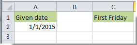
Till exempel finns det ett visst datum 1/1/2015 lokaliserar i cell A2 som bilden nedan visas. Om du vill hitta den första fredagen i månaden baserat på det angivna datumet, gör så här.

1. Välj en cell för att visa resultatet. Här väljer vi cellen C2.

2. Kopiera och klistra in formeln nedan i den och tryck sedan på ange nyckel.

=CEILING(EOMONTH(A2,-1)-5,7)+6

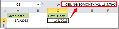
Då visas datumet i cell C2, det betyder att den första fredagen i januari 2015 är datum 1/2/2015.

Anmärkningar:

1. Om du vill hitta den första fredagen i andra månader, ange det angivna datumet för den månaden i cell A2 och använd sedan formeln.

2. I formeln är A2 referenscellen som det angivna datumet lokaliserar. Du kan ändra den för att tillgodose dina behov.

Hitta den sista fredagen i en månad

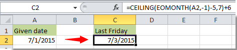
Det angivna datumet 1/1/2015 lokaliseras i cell A2, för att hitta den sista fredagen i denna månad i Excel, gör så här.

1. Välj en cell, kopiera formeln nedan till den och tryck sedan på ange för att få resultatet.

=DATE(YEAR(A2),MONTH(A2)+1,0)+MOD(-WEEKDAY(DATE(YEAR(A2),MONTH(A2)+1,0),2)-2,-7)

Sedan visar den sista fredagen i januari 2015 cellen B2.

Anmärkningar: Du kan ändra A2 i formeln till referenscellen för ditt angivna datum.


Relaterade artiklar:

Bästa kontorsproduktivitetsverktyg

🤖 Kutools AI Aide: Revolutionera dataanalys baserat på: Intelligent utförande   |  Generera kod  |  Skapa anpassade formler  |  Analysera data och generera diagram  |  Anropa Kutools funktioner.
Populära funktioner: Hitta, markera eller identifiera dubbletter   |  Ta bort tomma rader   |  Kombinera kolumner eller celler utan att förlora data   |   Rund utan formel ...
Superuppslag: Flera kriterier VLookup    VLookup med flera värden  |   VSök över flera ark   |   Fuzzy Lookup ....
Avancerad rullgardinslista: Skapa snabbt en rullgardinslista   |  Beroende rullgardinslista   |  Flervals-rullgardinslista ....
Kolumnhanterare: Lägg till ett specifikt antal kolumner  |  Flytta kolumner  |  Växla synlighetsstatus för dolda kolumner  |  Jämför intervall och kolumner ...
Utvalda funktioner: Rutnätsfokus   |  Designvy   |   Stor formelbar    Arbetsbok & Bladhanterare   |  Resursbibliotek (Automatisk text)   |  Datumväljare   |  Kombinera arbetsblad   |  Kryptera/Dekryptera celler    Skicka e-postmeddelanden efter lista   |  Superfilter   |   Specialfilter (filtrera fet/kursiv/genomstruken...) ...
Topp 15 verktygssatser12 text verktyg (lägga till text, Ta bort tecken, ...)   |   50+ Diagram Typer (Gantt Chart, ...)   |   40+ Praktiskt Formler (Beräkna ålder baserat på födelsedag, ...)   |   19 Införande verktyg (Infoga QR-kod, Infoga bild från sökväg, ...)   |   12 Konvertering verktyg (Siffror till ord, Valutaväxling, ...)   |   7 Slå ihop och dela verktyg (Avancerade kombinera rader, Dela celler, ...)   |   ... och mer

Uppgradera dina Excel-färdigheter med Kutools för Excel och upplev effektivitet som aldrig förr. Kutools för Excel erbjuder över 300 avancerade funktioner för att öka produktiviteten och spara tid.  Klicka här för att få den funktion du behöver mest...

Beskrivning


Fliken Office ger ett flikgränssnitt till Office och gör ditt arbete mycket enklare

  • Aktivera flikredigering och läsning i Word, Excel, PowerPoint, Publisher, Access, Visio och Project.
  • Öppna och skapa flera dokument i nya flikar i samma fönster, snarare än i nya fönster.
  • Ökar din produktivitet med 50 % och minskar hundratals musklick för dig varje dag!
Comments (12)
Rated 5 out of 5 · 1 ratings
This comment was minimized by the moderator on the site
Even shorter 😅
=lambda(Date;WeekDay;EOMONTH(Date;0)-WEEKDAY(EOMONTH(Date;0);WeekDay+10)+1
Where "WeekDay" parameter is 1=Monday, 7=Sunday
This comment was minimized by the moderator on the site
=lambda(Date;WeekDay;EOMONTH(Date;0)-WEEKDAY(EOMONTH(Date;0);WeekDay+10)+1)

I forgot a bracket at the end
This comment was minimized by the moderator on the site
Vậy công thức tính thứ sáu tuần thứ 2 của tháng như thế nào vậy ban?
This comment was minimized by the moderator on the site
Hi Tâm Cao Điền,
Suppose you want to calculate the second friday of the month based on the given date in A1, you can try the following formula:
=A18-DAY(A18)+CHOOSE(WEEKDAY(A18-DAY(A18),2),11,10,9,8,14,13,12)
This comment was minimized by the moderator on the site
porque cuando lo pruebo tal cual me sale error ?
o sea estoy copiando y pegando y no funciona

alguien sabe?
This comment was minimized by the moderator on the site
Hi andre,
Can you tell me which formula you used in the post? And what error your are experiencing?
This comment was minimized by the moderator on the site
Why not make the "last Friday" formula: =CEILING(EOMONTH(A2,0)-5,7)-1? That works for all dates I have tried....
This comment was minimized by the moderator on the site
Hi Eric,
I hop you are still on this forum and receive my reply.
Thanks so much for an EASY formula. I've never encountered =CEILING.
Rated 5 out of 5
This comment was minimized by the moderator on the site
Hi Eric,
Thanks for sharing it.
This comment was minimized by the moderator on the site
Hello and thank you for this formula. I am not an Excel guru and acnnot easily work out how to change this formula for the last Friday to be the Last Monday, or any other day. Can you please explain how to interpret this.
This comment was minimized by the moderator on the site
Matt,

The way the formula works is: First we find the last day of the month with the EOMONTH() function. For the last day of the current month, we use "0" as the month offset. For the previous month, it would be -1. (Either "=EOMONTH(A2,0)" or "=EOMONTH(A2,-1)".)

Then, in the "=CEILING()" function, we subtract the number of days required to bring us back to Sunday from the day for which we are searching. (For Tuesday, it would be -2, so we make the formula so far: "=CEILING(EOMONTH(A2,0)-2...."

We use the "significance" value of "7" because weeks are seven days long (of course).This finds the date of either the previous Saturday, or the following Saturday (Excel dates started with 1/1/1900, which was a Sunday. So if you enter a "1" in cell A2 with the Long Date format, the cell would read: "Sunday, January 1, 1900".). For that reason, the =CEILING() function, using "7" as the "significance" argument returns Saturday, which is always a multiple of 7 in Excel. Now the formula is "=CEILING(EOMONTH(A2,0)-2,7...".

Now we need to return the date to a Tuesday, so we either subtract 4 for the last Tuesday of the month, or add 3 for the first Tuesday of the next month. So the final formula is, respectively, either "=CEILING(EOMONTH(A2,0)-2,7)-4" or "=CEILING(EOMONTH(A2,0)-2,7)+3".

We can work through the math by assuming the last day of the month is either a Monday (assume its value is 9 - for ease of illustration, so the values do not go negative) or a Wednesday (assume value 11). "EOMONTH()" will return either of those days (9 or 11). Subtracting 2 results in the previous Saturday (value 7) or Monday (value 9), respectively. The CEILING() function then returns, respectively, the previous Saturday (value 7, because the ceiling of 7 with significance 7 is 7) or the current Saturday (value 14, because the ceiling of 9, significance 7, is 14). Subtracting 4 results in the previous Tuesday (value 3) or the current week's Tuesday (value 10), respectively. For the first Tuesday of the following month, adding 3 to the Saturday value (7 or 14) returns either Tuesday value 10, or Tuesday value 17, respectively.


Hopefully that helps you understand so that you can modify the formula as necessary. You can even change it to find the second Tuesday, or second to last Tuesday, by adding or subtracting an additional 7, respectively.
This comment was minimized by the moderator on the site
Hi Matt,
You just need to change the last number -7 to -1 to solove the problem.
=DATE(YEAR(A2),MONTH(A2)+1,0)+MOD(-WEEKDAY(DATE(YEAR(A2),MONTH(A2)+1,0),2)-2,-1)
There are no comments posted here yet
Please leave your comments in English
Posting as Guest
×
Rate this post:
0   Characters
Suggested Locations