Hoppa till huvudinnehåll

Hur visar jag motsvarande namn för den högsta poängen i Excel?

Antag att jag har ett utbud av data som innehåller två kolumner - namnkolumn och motsvarande poängkolumn, nu vill jag få namnet på den person som fick högst poäng. Finns det några bra sätt att hantera detta problem snabbt i Excel?

Visa motsvarande namn på högsta poäng med formler


pil blå höger bubbla Visa motsvarande namn på högsta poäng med formler

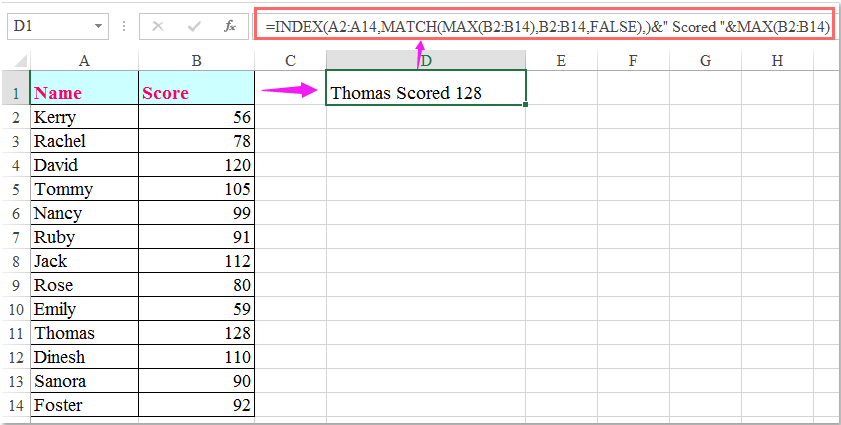
För att hämta namnet på den person som fick högst, kan följande formler hjälpa dig att få utdata.

Ange denna formel: =INDEX(A2:A14,MATCH(MAX(B2:B14),B2:B14,FALSE),)&" Scored "&MAX(B2:B14) till en tom cell där du vill visa namnet och tryck sedan på ange för att returnera resultatet enligt följande:

doc visningsnamn högsta poäng 1

Anmärkningar:

1. I ovanstående formel, A2: A14 är namnlistan som du vill hämta namnet från, och B2: B14 är poänglistan.

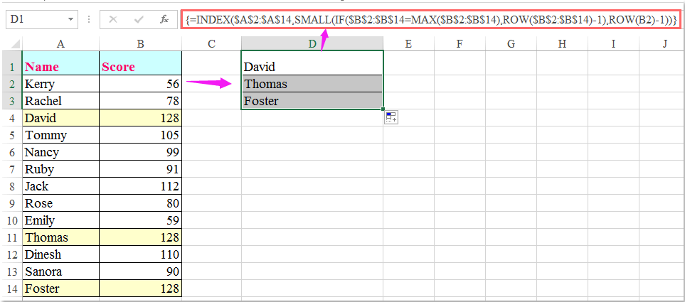
2. Ovanstående formel kan bara få förnamnet om det finns fler än ett namn med samma högsta poäng, för att få alla namn som fick högst poäng, kan följande matrisformel göra dig en tjänst.

Ange denna formel:

=INDEX($A$2:$A$14,SMALL(IF($B$2:$B$14=MAX($B$2:$B$14),ROW($B$2:$B$14)-1),ROW(B2)-1)), och tryck sedan på Ctrl + Skift + Enter tangenter tillsammans för att visa förnamnet, välj sedan formelcellen och dra ned fyllningshandtaget tills felvärdet visas, alla namn som fick högst poäng visas som nedan skärmdump:

doc visningsnamn högsta poäng 2

Bästa kontorsproduktivitetsverktyg

🤖 Kutools AI Aide: Revolutionera dataanalys baserat på: Intelligent utförande   |  Generera kod  |  Skapa anpassade formler  |  Analysera data och generera diagram  |  Anropa Kutools funktioner.
Populära funktioner: Hitta, markera eller identifiera dubbletter   |  Ta bort tomma rader   |  Kombinera kolumner eller celler utan att förlora data   |   Rund utan formel ...
Superuppslag: Flera kriterier VLookup    VLookup med flera värden  |   VSök över flera ark   |   Fuzzy Lookup ....
Avancerad rullgardinslista: Skapa snabbt en rullgardinslista   |  Beroende rullgardinslista   |  Flervals-rullgardinslista ....
Kolumnhanterare: Lägg till ett specifikt antal kolumner  |  Flytta kolumner  |  Växla synlighetsstatus för dolda kolumner  |  Jämför intervall och kolumner ...
Utvalda funktioner: Rutnätsfokus   |  Designvy   |   Stor formelbar    Arbetsbok & Bladhanterare   |  Resursbibliotek (Automatisk text)   |  Datumväljare   |  Kombinera arbetsblad   |  Kryptera/Dekryptera celler    Skicka e-postmeddelanden efter lista   |  Superfilter   |   Specialfilter (filtrera fet/kursiv/genomstruken...) ...
Topp 15 verktygssatser12 text verktyg (lägga till text, Ta bort tecken, ...)   |   50+ Diagram Typer (Gantt Chart, ...)   |   40+ Praktiskt Formler (Beräkna ålder baserat på födelsedag, ...)   |   19 Införande verktyg (Infoga QR-kod, Infoga bild från sökväg, ...)   |   12 Konvertering verktyg (Siffror till ord, Valutaväxling, ...)   |   7 Slå ihop och dela verktyg (Avancerade kombinera rader, Dela celler, ...)   |   ... och mer

Uppgradera dina Excel-färdigheter med Kutools för Excel och upplev effektivitet som aldrig förr. Kutools för Excel erbjuder över 300 avancerade funktioner för att öka produktiviteten och spara tid.  Klicka här för att få den funktion du behöver mest...

Beskrivning


Fliken Office ger ett flikgränssnitt till Office och gör ditt arbete mycket enklare

  • Aktivera flikredigering och läsning i Word, Excel, PowerPoint, Publisher, Access, Visio och Project.
  • Öppna och skapa flera dokument i nya flikar i samma fönster, snarare än i nya fönster.
  • Ökar din produktivitet med 50 % och minskar hundratals musklick för dig varje dag!
Comments (17)
No ratings yet. Be the first to rate!
This comment was minimized by the moderator on the site
Hi sir, I tried this method, But the problem is if top two students have the same score when I look for the highest 3 one student's name alone is repeated twice with the same score instead of second student's name. How to solve this.
This comment was minimized by the moderator on the site
Hello, Divyanathan
Maybe the following array formula can help you:

=IFERROR(INDEX(A:A,SUM(IF(($B$2:$B$100+ROUND(0.1/ROW($B$2:$B$100),5))=LARGE($B$2:$B$100+ROUND(0.1/ROW($B$2:$B$100),5),ROW(A1)),ROW($B$2:$B$100)))),"")


Note: After inserting the formula, please press Ctrl + Shift + Enter keys together to get the first result, and then drga this formula cell down to get the largest n results as you need.

Please have a try, hope it can help you!
This comment was minimized by the moderator on the site
Hola disculpa me podrías apoyar para sacar la formula o otro tipo de dato que me pueda dar el nombre del tota de un resultado?

explico tengo una tabla con 4 nombres diferentes distribuidos en las celdas C3,D3,E3 y F3 de las cuales cada celda mencionada tiene rangos de productos ejemplo: detergentes
y cada celda mencionada tiene precios diferentes.
en el resultado que debo de mostrar es el valor mínimo de precio de cada detergente de las celdas ya mencionadas arriba, y a lo que quiero llegar es que indique una formula o un dato que indique que en cada resultado a la derecho me indique el nombre del valor de resultado.
muestro un ejemplo mas especifico: en la celda <C3> tiene un nombre de insumos, en la celda C4 hasta C120 están los precios de cada detergente que maneja la celda C3, en la celda <D3> esta un nombre de biodetergentes, y mismo proceso la celda D4 hasta D120 están los precios en la celda G4 se encuentra el resultado del valor mínimo de estos dos nombres (insumos-biodetergentes) teniendo el valor menor el de nombre de insumos. ahora en la celda H4 quiero que me aparezca el nombre del valor de resultado en este caso que me aparezca el nombre de "insumos" como puedo hacer para que me aparezca este nombre? espero me allá podido dar a entender de lo que requiero
muchas gracias por su atención
saludos cordiales.
This comment was minimized by the moderator on the site
ik heb het ook geprobeerd met alle dezelfde gegevens zoals in het voorbeeld maar het werkt totaal niet
This comment was minimized by the moderator on the site
Hello jac, Sorry to hear that. As I have answered in the below comment, the two formulas work great for me. And I have been wondering why the formulas aren't working for the readers. There are two reasons that can lead to the malfunction of the second formula. 
First, if you are using Excel versions before Excel 2020, then you must enter the formula =INDEX($A$2:$A$14,SMALL(IF($B$2:$B$14=MAX($B$2:$B$14),ROW($B$2:$B$14)-1),ROW(B2)-1)) via pressing Ctrl + Shift + Enter keys together.
Second, When you get the first result, remember to select the formula cell and drag the fill handle down until error value appears. So all the other results will be returned.
And as you can see in the screenshots below, the two formulas are working fine for me.  Hope my solution works. Have a nice day.
Sincerely,Mandy
This comment was minimized by the moderator on the site
bullshitdoes not work
This comment was minimized by the moderator on the site
Hello,
Sorry to hear that. But I did tried the two formulas in the article and both of them works perfectly. Please see the screenshots I uploaded here. And we would love to solve the problem for you if you can provide the details of the problem. Looking forward to your reply.Sincerely,Mandy
This comment was minimized by the moderator on the site
Trying to do the same thing but with the minimum score in Microsoft sheets. I swapped max for min as below and it didn't work =INDEX($A$2:$A$14,SMALL(IF($B$2:$B$14=MIN($B$2:$B$14),ROW($B$2:$B$14)-1),ROW(B2)-1))
This comment was minimized by the moderator on the site
Hi. This formula was exactly what I was looking for. However is there a way do this with the lowest Score but above 0 (in my case £00.00) I removed the bit of formula that displays the amount as only needed the Name and comment.I changed the MAX for MIN but there are a few entries at 0 (£00.00) and formula displays the name for the first of the '0' entries
This comment was minimized by the moderator on the site
Hello, Nigel,To lookup the lowest value above 0, you should apply the below array formula:After entering the formula, please remember to press Ctrl + Shift + Enter keys together to get the correct result.=INDEX(A2:A8,MATCH(MIN(IF(B2:B8>0,B2:B8)),B2:B8,0))&" Scored "&MIN(IF(B2:B8>0,B2:B8))
Please try, hope it can help you!
This comment was minimized by the moderator on the site
How do you find the second highest student? Please help me :( I only get the name of Thomas.
This comment was minimized by the moderator on the site
How do you find the second highest student?
This comment was minimized by the moderator on the site
How would you show two names if the high scores match?
This comment was minimized by the moderator on the site
Hello, Chris,
To get all names if there are multiple high scores match, the second formula in this article can do you a favor.
Please try it, thank you!
This comment was minimized by the moderator on the site
How would you get the matching numbers with the corresponding names to display horizontally?
There are no comments posted here yet
Load More
Please leave your comments in English
Posting as Guest
×
Rate this post:
0   Characters
Suggested Locations