Hoppa till huvudinnehåll

Hur hanterar jag om cellen innehåller ett ord, lägg sedan en text i en annan cell?

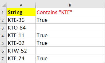
Här är en lista över produkt-ID, och nu vill jag ta reda på om cellen innehåller en sträng "KTE", och lägg sedan texten "TRUE" i dess intilliggande cell enligt nedanstående skärmdump. Har du några snabba sätt att lösa det? I den här artikeln pratar jag om knep för att hitta om en cell innehåller ett ord och sedan lägga en text i den intilliggande cellen.


Om en cell innehåller ett ord motsvarar en annan cell en specifik text

Här är en enkel formel som kan hjälpa dig att snabbt kontrollera om en cell innehåller ett ord och sedan lägga en text i nästa cell.

Välj den cell du vill lägga till texten och skriv den här formeln = IF (ISNUMBER (SÖK ("KTE", A2)), "True", "") och dra sedan handtaget för automatisk fyllning ner till cellerna du vill använda denna formel. Se skärmdump:

doc om cellen innehåller ett ord är lika med 8 skottpil höger doc om cellen innehåller ett ord är lika med 9


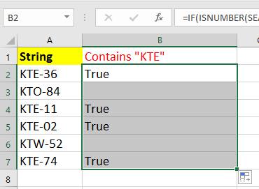
I formeln är A2 den cell som du vill kontrollera om innehåller ett specifikt ord, och KTE är det ord du vill kontrollera, True är texten du vill visa i en annan cell. Du kan ändra dessa referenser efter behov.


Välj eller markera om en cell innehåller ett ord

Om du vill kontrollera om en cell innehåller ett specifikt ord och sedan markera eller markera det kan du använda Välj specifika celler egenskap av Kutools för Excel, som snabbt kan hantera detta jobb.

Kutools för Excel, med mer än 300 praktiska funktioner, underlättar dina jobb. 

När du har installerat Kutools för Excel, gör så här :(Gratis nedladdning Kutools för Excel nu!)

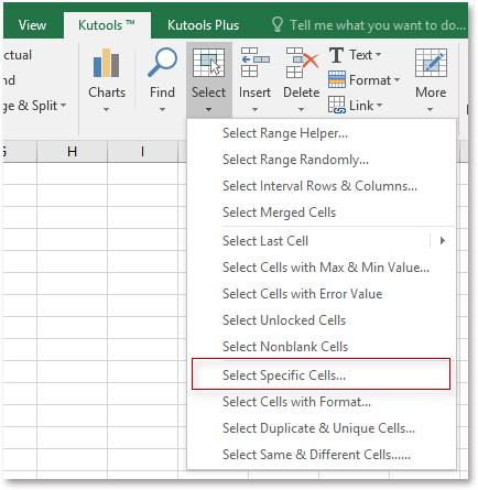
1. Välj det intervall du vill kontrollera om cellen innehåller ett specifikt ord och klicka Kutools > Välja > Välj specifika celler. Se skärmdump:

doc om cellen innehåller ett ord är lika med 3

2. Kontrollera sedan i poppdialogen Cell alternativ och välj innehåller från den första rullgardinsmenyn och skriv sedan ordet du vill kontrollera i nästa textruta. Se skärmdump:
doc om cellen innehåller ett ord är lika med 4

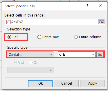
3. klick Ok, en dialogruta dyker upp för att påminna dig om hur celler kan innehålla ordet du vill hitta och klicka OK för att stänga dialogen. Se skärmdump:
doc om cellen innehåller ett ord är lika med 5

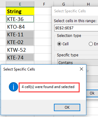
4. Sedan har cellerna som innehåller det angivna ordet valts, om du vill markera dem, gå till Hem > Fyllningsfärg att välja en fyllningsfärg för att utmärka dem.
doc om cellen innehåller ett ord är lika med 6

Tips. Om du vill ha en gratis testversion av Välj specifika celler fungera, gå till gratis nedladdning Kutools för Excel först och sedan tillämpa operationen enligt ovanstående steg.

Bästa kontorsproduktivitetsverktyg

🤖 Kutools AI Aide: Revolutionera dataanalys baserat på: Intelligent utförande   |  Generera kod  |  Skapa anpassade formler  |  Analysera data och generera diagram  |  Anropa Kutools funktioner.
Populära funktioner: Hitta, markera eller identifiera dubbletter   |  Ta bort tomma rader   |  Kombinera kolumner eller celler utan att förlora data   |   Rund utan formel ...
Superuppslag: Flera kriterier VLookup    VLookup med flera värden  |   VSök över flera ark   |   Fuzzy Lookup ....
Avancerad rullgardinslista: Skapa snabbt en rullgardinslista   |  Beroende rullgardinslista   |  Flervals-rullgardinslista ....
Kolumnhanterare: Lägg till ett specifikt antal kolumner  |  Flytta kolumner  |  Växla synlighetsstatus för dolda kolumner  |  Jämför intervall och kolumner ...
Utvalda funktioner: Rutnätsfokus   |  Designvy   |   Stor formelbar    Arbetsbok & Bladhanterare   |  Resursbibliotek (Automatisk text)   |  Datumväljare   |  Kombinera arbetsblad   |  Kryptera/Dekryptera celler    Skicka e-postmeddelanden efter lista   |  Superfilter   |   Specialfilter (filtrera fet/kursiv/genomstruken...) ...
Topp 15 verktygssatser12 text verktyg (lägga till text, Ta bort tecken, ...)   |   50+ Diagram Typer (Gantt Chart, ...)   |   40+ Praktiskt Formler (Beräkna ålder baserat på födelsedag, ...)   |   19 Införande verktyg (Infoga QR-kod, Infoga bild från sökväg, ...)   |   12 Konvertering verktyg (Siffror till ord, Valutaväxling, ...)   |   7 Slå ihop och dela verktyg (Avancerade kombinera rader, Dela celler, ...)   |   ... och mer

Uppgradera dina Excel-färdigheter med Kutools för Excel och upplev effektivitet som aldrig förr. Kutools för Excel erbjuder över 300 avancerade funktioner för att öka produktiviteten och spara tid.  Klicka här för att få den funktion du behöver mest...

Beskrivning


Fliken Office ger ett flikgränssnitt till Office och gör ditt arbete mycket enklare

  • Aktivera flikredigering och läsning i Word, Excel, PowerPoint, Publisher, Access, Visio och Project.
  • Öppna och skapa flera dokument i nya flikar i samma fönster, snarare än i nya fönster.
  • Ökar din produktivitet med 50 % och minskar hundratals musklick för dig varje dag!
Comments (21)
No ratings yet. Be the first to rate!
This comment was minimized by the moderator on the site
Buenas noches,

Tengo una columna con varias categorías de tareas (administrativo, profesor, etc) y quiero armar la columna siguiente indicando si es x tarea que sea nivel alto, si es otra Medio y así. Intenté con la fórmula SI y SI. CONJUNTO pero no parece funcionar cuando no hay valores numéricos. Vi ejemplos pero con si C2 es mayor que entonces tal palabra...
This comment was minimized by the moderator on the site
Buen día, disculpa, queria ver si me puedes ayudar con una formula.

En una celda tengo una oracion, y quiero que la celda de un lado me escriba cierta letra o palabra cuando en la primera celda tenga alguna palabra.

Ejemplo
en la celda A1 tengo una oracion: papa manzana pasta, lechuga.
en la celda A2 tengo: papa manzana, zanahoria, lechuga.

Quiero que en la celda B1 me aparezca la palabra "ensalada" solo porque en la A1 tiene "lechuga"
y en la celda B2 me aparezca la palabra: "arbol" porque tiene la palabra "manzana"

Nota quiero que de prioridad a la lechuga antes que a la manzana
Sino se puede dar prioridad entonces digamos que quitamos la palabra "manzana" de la primera oracion


No se si me di a entender, no se me ocurrio como dar el ejemplo
This comment was minimized by the moderator on the site
Hi, luis, here is a formula may help you.
Take an example for explaining the formula, if cell contains "KTE" then returns "Y", if cell contains "KTW" then returns "T", if cell contains both of "KTE' and "KTW" then returns "Y".
=IF(AND(ISNUMBER(SEARCH("KTE",A3)), ISNUMBER(SEARCH("KTW",A3)) ),"Y", IF(ISNUMBER(SEARCH("KTE",A3)), "Y", IF(ISNUMBER(SEARCH("KTW",A3)), "T", "")))
change the reference and the values as you need.
https://www.extendoffice.com/images/stories/comments/sun-comment/doc-return-value-based-on-word.png
Tip: If you in spanish version, maybe need to change the formula to spanish formula.
This comment was minimized by the moderator on the site
How do you keep this going, if I have 5 other unique labels that need to spit out 5 other unique corresponding phrases?
This comment was minimized by the moderator on the site
Hi, Andy, yes, you need to use 5 different formulas to acheive your purpose.
This comment was minimized by the moderator on the site
kolom satu
adam
andi
budi
dst

kolom dua
andi jaya
budiarto
adam malik
dst


kolom 3 (hasil pakai rumus)


pertanyaan:
bagaimana rumus di kolom 3, jika kita ingin memunculkan nama kolom 2 dikolom 3 yg mengandung teks di kolom satu.

saya minta petunjuk dari para pakar excel.

Terima kasih
Andi
This comment was minimized by the moderator on the site
Hi, Andi, I realy like to help you, but I cannot read your language, could you login and upload a screenshot to show the result you want? Then I will try to find method to solve it.
This comment was minimized by the moderator on the site
kolom satu kolom dua kolom 3 (hasil rumus)
adam andi jaya
andi budiarto
budi adam malik
dst dst

bagaimana rumus di kolom 3, jika kita ingin memunculkan nama kolom 2 dikolom 3 yg mengandung teks di kolom satu.

saya minta petunjuk dari para pakar excel.

Terima kasih
Andi
This comment was minimized by the moderator on the site
If column has text, alpha-numeric & numeric values, using the convert tool does not apply the text values to numeric. Makes sense. Though, how could you configure a IF Vlookup to compensate if a cell has text?
This comment was minimized by the moderator on the site
Sorry, which convert tool you mean? The formula can work correctly whatever the column contains alpha, alpha-numeric or numeric string.
This comment was minimized by the moderator on the site
Hello,

Question. If I need this formula to apply to two different returns. For example, if a cell contains the word "Senior", another cell would return "32" and if the cell contains "Associate" then the other cell would return 16.
This comment was minimized by the moderator on the site
Here's the formula. Assume there's a list of titles starting in cell A2:

Senior Engineer
Associate Engineer
Senior Engineer
Senior Engineer
Vice President
Associate Engineer
Associate Engineer
Senior Vice Presdent

In cell B2 (or whatever cell you wish to populate with the results), write:

=IF(ISNUMBER(FIND("Senior",A2)),"32",IF(ISNUMBER(FIND("Associate",A2)),"16"))

You could check for additional values by adding additional nested IF statements.
This comment was minimized by the moderator on the site
Sorry I cannot figore out the correct formula to solve your problem, you can go to our forum https://www.extendoffice.com/forum.html to place your question, maybe someone can help you.
This comment was minimized by the moderator on the site
Thanks for this. Can this code be edited so that instead of placing specific text beside the source text, it can be formatted to place the text in a different cell?
This comment was minimized by the moderator on the site
i know what u mean. i need this function to.
This comment was minimized by the moderator on the site
Do you mean to extract the text in different cell while the cell contains the specifict text as below screenshot shown?
This comment was minimized by the moderator on the site
Sorry, I do not realy understand your question. Could you give me more detail description?
This comment was minimized by the moderator on the site
How would you write the formula is you have text-text-text and you want to pull the final text? AB-GUFJ-CD if you want to pull the CD?
This comment was minimized by the moderator on the site
Hello, this formula may help you =TRIM(RIGHT(SUBSTITUTE(A12,"-",REPT(" ",255)),255)), A12 is the text string you use, change it as you need. If it works, please let me know. Thanks.
This comment was minimized by the moderator on the site
LOL ...did you mean True?
This comment was minimized by the moderator on the site
Embarrrassed...yes, I mean true~~, I have rewrote it, thank u for ur remind.
There are no comments posted here yet
Please leave your comments in English
Posting as Guest
×
Rate this post:
0   Characters
Suggested Locations