Hoppa till huvudinnehåll

Hur villkorlig formatering baserat på ett annat ark i Google-ark?

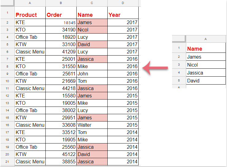
Om du vill använda den villkorliga formateringen för att markera celler baserat på en lista med data från ett annat ark som följande skärmdump som visas i Google-ark, har du några enkla och bra metoder för att lösa det?

Villkorlig formatering för att markera celler baserat på en lista från ett annat ark i Google Sheets


Villkorlig formatering för att markera celler baserat på en lista från ett annat ark i Google Sheets


Gör med följande steg för att slutföra det här jobbet:

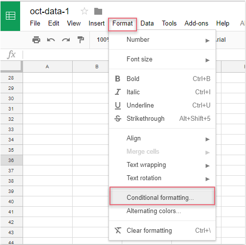
1. Klicka bildad > Villkorlig formatering, se skärmdump:

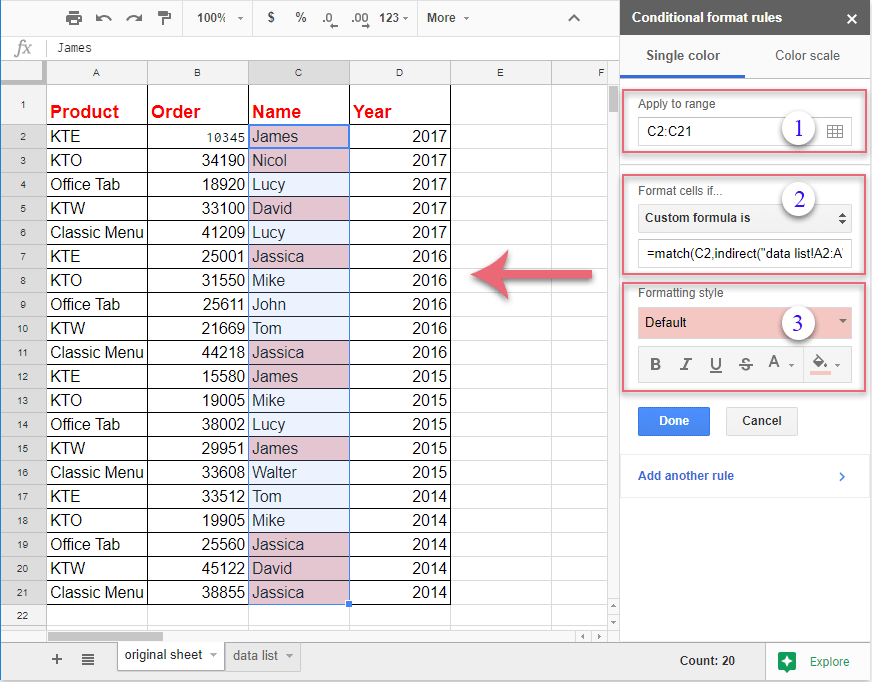
2. I Regler för villkorligt format i rutan, gör följande:

(1.) Klicka på -knappen för att välja kolumndata som du vill markera;

(2.) I Formatera celler om rullgardinsmeny, välj Anpassad formel är och ange sedan denna formel: = matchning (C2, indirekt ("datalista! A2: A"), 0) i textrutan;

(3.) Välj sedan en formatering från Formateringsstil som du behöver.

Anmärkningar: I ovanstående formel: C2 är den första cellen i kolumndata som du vill markera och datalista! A2: A är arknamnet och listcellområdet som innehåller de kriterier du vill markera cellerna baserat på.

3. Och alla matchande celler baserade på listcellerna har markerats på en gång, sedan ska du klicka på Färdig knappen för att stänga Regler för villkorligt format ruta som du behöver.


Bästa kontorsproduktivitetsverktyg

🤖 Kutools AI Aide: Revolutionera dataanalys baserat på: Intelligent utförande   |  Generera kod  |  Skapa anpassade formler  |  Analysera data och generera diagram  |  Anropa Kutools funktioner.
Populära funktioner: Hitta, markera eller identifiera dubbletter   |  Ta bort tomma rader   |  Kombinera kolumner eller celler utan att förlora data   |   Rund utan formel ...
Superuppslag: Flera kriterier VLookup    VLookup med flera värden  |   VSök över flera ark   |   Fuzzy Lookup ....
Avancerad rullgardinslista: Skapa snabbt en rullgardinslista   |  Beroende rullgardinslista   |  Flervals-rullgardinslista ....
Kolumnhanterare: Lägg till ett specifikt antal kolumner  |  Flytta kolumner  |  Växla synlighetsstatus för dolda kolumner  |  Jämför intervall och kolumner ...
Utvalda funktioner: Rutnätsfokus   |  Designvy   |   Stor formelbar    Arbetsbok & Bladhanterare   |  Resursbibliotek (Automatisk text)   |  Datumväljare   |  Kombinera arbetsblad   |  Kryptera/Dekryptera celler    Skicka e-postmeddelanden efter lista   |  Superfilter   |   Specialfilter (filtrera fet/kursiv/genomstruken...) ...
Topp 15 verktygssatser12 text verktyg (lägga till text, Ta bort tecken, ...)   |   50+ Diagram Typer (Gantt Chart, ...)   |   40+ Praktiskt Formler (Beräkna ålder baserat på födelsedag, ...)   |   19 Införande verktyg (Infoga QR-kod, Infoga bild från sökväg, ...)   |   12 Konvertering verktyg (Siffror till ord, Valutaväxling, ...)   |   7 Slå ihop och dela verktyg (Avancerade kombinera rader, Dela celler, ...)   |   ... och mer

Uppgradera dina Excel-färdigheter med Kutools för Excel och upplev effektivitet som aldrig förr. Kutools för Excel erbjuder över 300 avancerade funktioner för att öka produktiviteten och spara tid.  Klicka här för att få den funktion du behöver mest...

Beskrivning


Fliken Office ger ett flikgränssnitt till Office och gör ditt arbete mycket enklare

  • Aktivera flikredigering och läsning i Word, Excel, PowerPoint, Publisher, Access, Visio och Project.
  • Öppna och skapa flera dokument i nya flikar i samma fönster, snarare än i nya fönster.
  • Ökar din produktivitet med 50 % och minskar hundratals musklick för dig varje dag!


Comments (27)
Rated 5 out of 5 · 2 ratings
This comment was minimized by the moderator on the site
Hi! skyyang ! Thank you, =match(C2,indirect("data list!A2:A"),0) works for me.

But I would like to format more than one column, so column A in sheet a is checked against column B in sheet b , and so.
There are so many columns so I can not apply one format per column, but a whole conditional format for the whole sheet.


How should I modify the range and the formula?

Thanks!
This comment was minimized by the moderator on the site
What if the cell values you're trying to match are hyperlinks?
Rated 5 out of 5
This comment was minimized by the moderator on the site
Pardon, il fallait lire =A1<>INDIRECT("PreviousVersion!"& CHAR (COLUMN () + 64) & ROW ()) ...
This comment was minimized by the moderator on the site
Bonjour,
J'ai une autre question du même type au sujet d'un formatage conditionnel qui fonctionne sur Excel mais que je n'arrive pas à porter sur Google Sheet :
L'idée est de comparer 2 versions d'une même feuille que l'on stock à l'aide de 2 onglets (2 feuilles du même workbook)

La formule est la suivante : =A1<>'previousVersion'!A1 avec un formatage fond jaune pour mettre en évidence les changements sur toute la feuille car l'idée est d'appliquer ce
formatage conditionnel sur toutes les cellules de la feuille ($A$1:$V:1000)

Sur Google sheet cette formule m'est interdite et si je passe par un "indirect("previousVersion!A1"), je perds le coté dynamique sur le "A1" de la feuille precious version
Si j'essaye =A1<>indirect("previousVersion!"&A1) j'ai une erreur car c'est la valeur de A1 qui est interprétée et concaténée avec "previousVersion!"

Si j'essaye la formule =C3<>INDIRECT("PreviousVersion!"& CHAR (COLUMN () + 64) & ROW ()) cela ne fonctionne pas non plus....

Si vous avez une solution...
Merci d'avance
This comment was minimized by the moderator on the site
Bonjour,
Dans Feuille google je cherche la formule suivante
Si dans la cel A1 = text alors dans la Cel B1 ecire telle valeur ou texte automatiquement
Merci d avance pour votre aide
This comment was minimized by the moderator on the site
What if it's not an exact match but contains the reference data.
This comment was minimized by the moderator on the site
Hello, ashley
To solve your problem, please apply the below formula:
=REGEXMATCH(C2:C21,INDIRECT("Sheet2!$A$2"))

Please try, hope it can help you!
This comment was minimized by the moderator on the site
What happens if the data in my list is in more than one column? When I try to use datalist!A2:M or datalist!A:M or datalist!A2:M17 none of those work.
This comment was minimized by the moderator on the site
I have even tried naming the specific range I want to refer to and using that in the formula, no luck.
This comment was minimized by the moderator on the site
How to highlight the entire row data with conditional formatting using other sub-sheet
This comment was minimized by the moderator on the site
Hello, Ranganath
To highlight the entire row based on the data list, please do as this:
1. In the Apply to range box, select the whole sheet;
2. Apply this formula: =match($C2,indirect("datalist!A2:A"),0) into the Custom formula is textbox.
Please try, hope it can help you!

https://www.extendoffice.com/images/stories/comments/comment-skyyang/doc-highlight-entire-row.png
This comment was minimized by the moderator on the site
Hey, Thanks for replying. I have tried the formula but its not working.
Rated 5 out of 5
This comment was minimized by the moderator on the site
Hi,
Have you modified the sheet name and cell reference to your own data?
$C2 is the first cell of the column data that you want to highlight, and the datalist!A2:A is another sheet name and list range which contains the criteria you want to highlight the cells based on.
Please check them, thank you!
This comment was minimized by the moderator on the site
This doesn't work for me. I have triple checked everything.

Apply to range: K1:K2158

=match(K2,indirect("TorontoCitys!A1:A"),0)

It highlights random other city names, not in the TorontoCity's list.

K2 (is my main sheet and the starting column cell of the column I want to be affected.
TorontoCitys (is the name of the sheet)
A1 is the start of the column of the list of city names.
A is the column.

Could be that my punctuation's are incorrect?

Thanks in advance.
This comment was minimized by the moderator on the site
Hello friend,

Glad to help. Your formula is correct, please don't worry. The problem is the range you apply to. It shouldn't be K1:K2158, but K2:K2158.

Please see the screenshots. The example is simple but enough to explain the problem.

The correct "Apply to Range" is A2:A20. And the correct formula is =match(A2,indirect("TorontoCitys!A1:A"),0). Then correct cities can be highlighted. Please see screenshot 2.
But if I change the "Apply to Range" to A1:A20, the wrong city name is highlighted. Please see screenshot 3.

So please change your "Apply to Range" from K1:K2158 to K2:K2158. The problem should be solved. Looking forward to your reply.

Sincerely,
Mandy
This comment was minimized by the moderator on the site
how do you do this but with the entire row highlighted
There are no comments posted here yet
Load More
Please leave your comments in English
Posting as Guest
×
Rate this post:
0   Characters
Suggested Locations