Hoppa till huvudinnehåll

Hur vlookup för att returnera flera kolumner från Excel-tabellen?

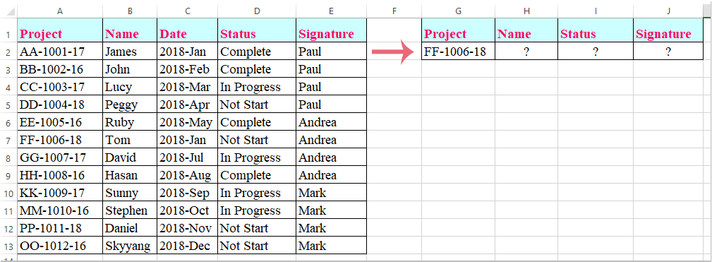
I Excel-kalkylbladet kan du använda Vlookup-funktionen för att returnera matchande värde från en kolumn. Men ibland kan du behöva extrahera matchade värden från flera kolumner enligt följande skärmdump. Hur kunde du få motsvarande värden samtidigt från flera kolumner med hjälp av Vlookup-funktionen?

doc vlookup flera kolumner 1

Vlookup för att returnera matchande värden från flera kolumner med matrisformel


Vlookup för att returnera matchande värden från flera kolumner med matrisformel

Här introducerar jag Vlookup-funktionen för att returnera matchade värden från flera kolumner, gör så här:

1. Välj cellerna där du vill placera matchande värden från flera kolumner, se skärmdump:

doc vlookup flera kolumner 2

2. Ange sedan denna formel: =VLOOKUP(G2,A1:E13,{2,4,5},FALSE) i formelfältet och tryck sedan på Ctrl + Skift + Enter nycklar tillsammans, och matchande värden från flera kolumner har extraherats på en gång, se skärmdump:

doc vlookup flera kolumner 3

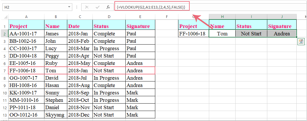
Anmärkningar: I ovanstående formel, G2 är kriterierna som du vill returnera värden baserat på, A1: E13 är det tabellintervall du vill söka efter, numret 2, 4, 5 är kolumnnumren som du vill returnera värden från.

Bästa kontorsproduktivitetsverktyg

🤖 Kutools AI Aide: Revolutionera dataanalys baserat på: Intelligent utförande   |  Generera kod  |  Skapa anpassade formler  |  Analysera data och generera diagram  |  Anropa Kutools funktioner.
Populära funktioner: Hitta, markera eller identifiera dubbletter   |  Ta bort tomma rader   |  Kombinera kolumner eller celler utan att förlora data   |   Rund utan formel ...
Superuppslag: Flera kriterier VLookup    VLookup med flera värden  |   VSök över flera ark   |   Fuzzy Lookup ....
Avancerad rullgardinslista: Skapa snabbt en rullgardinslista   |  Beroende rullgardinslista   |  Flervals-rullgardinslista ....
Kolumnhanterare: Lägg till ett specifikt antal kolumner  |  Flytta kolumner  |  Växla synlighetsstatus för dolda kolumner  |  Jämför intervall och kolumner ...
Utvalda funktioner: Rutnätsfokus   |  Designvy   |   Stor formelbar    Arbetsbok & Bladhanterare   |  Resursbibliotek (Automatisk text)   |  Datumväljare   |  Kombinera arbetsblad   |  Kryptera/Dekryptera celler    Skicka e-postmeddelanden efter lista   |  Superfilter   |   Specialfilter (filtrera fet/kursiv/genomstruken...) ...
Topp 15 verktygssatser12 text verktyg (lägga till text, Ta bort tecken, ...)   |   50+ Diagram Typer (Gantt Chart, ...)   |   40+ Praktiskt Formler (Beräkna ålder baserat på födelsedag, ...)   |   19 Införande verktyg (Infoga QR-kod, Infoga bild från sökväg, ...)   |   12 Konvertering verktyg (Siffror till ord, Valutaväxling, ...)   |   7 Slå ihop och dela verktyg (Avancerade kombinera rader, Dela celler, ...)   |   ... och mer

Uppgradera dina Excel-färdigheter med Kutools för Excel och upplev effektivitet som aldrig förr. Kutools för Excel erbjuder över 300 avancerade funktioner för att öka produktiviteten och spara tid.  Klicka här för att få den funktion du behöver mest...

Beskrivning


Fliken Office ger ett flikgränssnitt till Office och gör ditt arbete mycket enklare

  • Aktivera flikredigering och läsning i Word, Excel, PowerPoint, Publisher, Access, Visio och Project.
  • Öppna och skapa flera dokument i nya flikar i samma fönster, snarare än i nya fönster.
  • Ökar din produktivitet med 50 % och minskar hundratals musklick för dig varje dag!
Comments (15)
No ratings yet. Be the first to rate!
This comment was minimized by the moderator on the site
how can i search for multiple lookup value?for eg: these two arrays shows diff freq coumn,gain,veritcal BW,tolerance etc.I want to get an average values gain and 3db BW..how can i enter the formula
y1    1800    7.5dBi +/- 2.9    22.1° +/- 6.8        7.5
y1    1900    7.6dBi +/- 3.0    18.9° +/- 3.6        7.6
y1    2100    6.7dBi +/- 2.6    17.7° +/- 3.6        6.7
y1    AWS    7.2dBi +/- 2.8    20.4° +/- 9.4        7.2
y1    2300    8.3dBi +/- 3.6    15.8° +/- 1.6        8.3
y1    2600    7.9dBi +/- 2.4    17.1° +/- 1.7        7.9
y2    1800    6.9dBi +/- 1.4    27.1° +/- 10.8        6.9
y2    1900    6.9dBi +/- 1.5    23.0° +/- 12.5        6.9
y2    2100    7.6dBi +/- 2.3    21.7° +/- 19.6        7.6
y2    AWS    8.0dBi +/- 2.5    23.3° +/- 13.8        8
y2    2300    7.7dBi +/- 1.6    15.9° +/- 5.9        7.7
y2    2600    6.5dBi +/- 2.3    14.5° +/- 3.9        6.5
This comment was minimized by the moderator on the site
I have many rows with same value but need to get multiple value after look up, I need to get two different EO ref , how can U##TRX EO
HXPRE-MQ1371 AB0024822
This comment was minimized by the moderator on the site
Thank you!! The { } of the columns is what I was missing. Appreciate this page!
This comment was minimized by the moderator on the site
Thanks! Super helpful, when other online options weren't
This comment was minimized by the moderator on the site
What if you need to have multiple rows as well? Ex. find all the FF-1006-18 rows while still only bringing back column B, D, and E.
This comment was minimized by the moderator on the site
Hello, Shelly,
Maybe there is not a direct formula for helping you, but, you can apply the below array fromula to get all matching values from the entire row, and then delete or hide the unwanted column as you need.
=INDEX($A$2:$E$10, SMALL(IF($G$2=$A$2:$A$10, ROW($A$2:$A$10)-MIN(ROW($A$2:$A$10))+1, ""), ROW(B1)),COLUMN(B1))
Then press Ctrl + Shift + Enter keys to get the first cell and then drag the fill handle to right and then drga down to get all corresponding values.

Please try, hope it can help you!
This comment was minimized by the moderator on the site
Thanks! This was really Helpful!
This comment was minimized by the moderator on the site
This method does not work. Even if it did, it is not the proper method.
Example of correct method is:
VLOOKUP($A2:$A1093, '[Workbook1.xlsx]Sheet2'!$A$2:$D$111,COLUMN(G2),FALSE)

Make sure you add $ before the column letter of your lookup reference to make sure it remains static, once done, using the filler button on the selected target cell, drag right to the corresponding number of columns.
This comment was minimized by the moderator on the site
This comment is exactly what I needed
This comment was minimized by the moderator on the site
How can I do this using 2 different spread sheets?
This comment was minimized by the moderator on the site
Hello, Lana,
The above formula in this article also can help you to get the results in another worksheet, you just need to change the cell reference as follows:
=VLOOKUP(A1,Sheet1!A1:E13,{2,4,5},FALSE)
Please remember to press Ctrl + Shift + Enter keys together to get the correct results.
This comment was minimized by the moderator on the site
NOT GETTING MULTIPLE COLUMN I'M GETTING ONLY ONE COLUMN VALUE
This comment was minimized by the moderator on the site
Hi, HARI,
To apply this formula, first, you should select the multiple cells where you want to output the results, and then copy the formula into the formula bar, then press Ctrl + Shift + Enter keys together to get the results.
Please try, hope it can help you!
This comment was minimized by the moderator on the site
This is great. How do I carry this formula down if I have 10,000 rows? I've tried a few ways but of course it's changing the formula on me.
This comment was minimized by the moderator on the site
Hi, Scully,
To apply this formula to multiple rows, you just need to change the relative cell reference to absolute reference, as this: =VLOOKUP(A1,Sheet1!$A$1:$E$13,{2,4,5},FALSE).
Please try this, hope it can help you!
There are no comments posted here yet
Please leave your comments in English
Posting as Guest
×
Rate this post:
0   Characters
Suggested Locations