Hoppa till huvudinnehåll

Hur skapar jag rullgardinslista med flera kryssrutor i Excel?

Många Excel-användare tenderar att skapa rullgardinslista med flera kryssrutor för att välja flera objekt från listan per gång. Du kan faktiskt inte skapa en lista med flera kryssrutor med datavalidering. I den här handledningen kommer vi att visa dig två metoder för att skapa rullgardinslista med flera kryssrutor i Excel.

Använd listrutan för att skapa en listruta med flera kryssrutor
A: Skapa en listruta med källdata
B: Namnge cellen där du hittar de valda objekten
C: Infoga en form som hjälper till att mata ut de valda objekten
Skapa enkelt listrutan med kryssrutor med ett fantastiskt verktyg
Fler handledning för rullgardinsmenyn ...


Använd listrutan för att skapa en listruta med flera kryssrutor

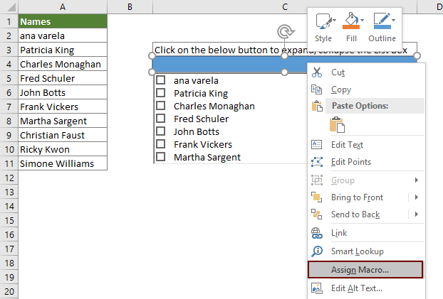
Som nedanstående skärmdump visas, i det aktuella kalkylbladet, kommer alla namn i intervall A2: A11 att vara källdata i listrutan. Klicka på knappen i cell C4 för att mata ut de valda objekten, och alla valda objekt i listrutan visas i cell E4. Gör så här för att uppnå detta.

A. Skapa en listruta med källdata

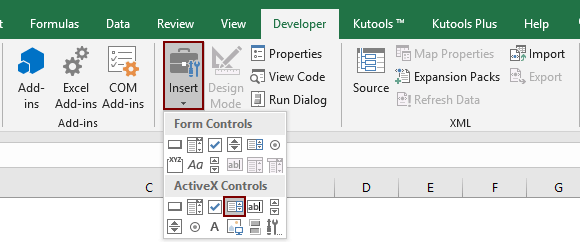
1. klick Utvecklare > Insert > Listbox (Active X Control). Se skärmdump:

2. Rita en listruta i det aktuella kalkylbladet, högerklicka på den och välj sedan Våra Bostäder från högerklickmenyn.

3. I Våra Bostäder i dialogrutan måste du konfigurera enligt följande.

  • 3.1 I ListFillRange rutan, ange källområdet du kommer att visa i listan (här anger jag intervall A2: A11);
  • 3.2 I Liststil rutan, välj 1 - fmList StyleOption;
  • 3.3 I Flera val rutan, välj 1 - fmMultiSelectMulti;
  • 3.4 Stäng Våra Bostäder dialog ruta. Se skärmdump:

B: Namnge cellen där du hittar de valda objekten

Om du behöver mata ut alla markerade objekt till en angiven cell som E4, gör så här.

1. Välj cellen E4, ange ListBoxOutput i Namn Box och tryck på ange nyckel.

C. Infoga en form som hjälper till att mata ut de markerade objekten

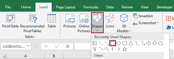
1. klick Insert > Former > Rektangel. Se skärmdump:

2. Rita en rektangel i ditt kalkylblad (här ritar jag rektangeln i cell C4). Högerklicka sedan på rektangeln och välj Tilldela makro från högerklickmenyn.

3. I Tilldela makro dialogrutan, klicka på Nya knapp.

4. I öppningen Microsoft Visual Basic för applikationer fönstret, byt ut den ursprungliga koden i Modulerna fönster med VBA-koden nedan.

VBA-kod: Skapa en lista med flera kryssrutor

Sub Rectangle1_Click()
'Updated by Extendoffice 20200730
Dim xSelShp As Shape, xSelLst As Variant, I, J As Integer
Dim xV As String
Set xSelShp = ActiveSheet.Shapes(Application.Caller)
Set xLstBox = ActiveSheet.ListBox1
If xLstBox.Visible = False Then
    xLstBox.Visible = True
    xSelShp.TextFrame2.TextRange.Characters.Text = "Pickup Options"
    xStr = ""
    xStr = Range("ListBoxOutput").Value
    
    If xStr <> "" Then
         xArr = Split(xStr, ";")
    For I = xLstBox.ListCount - 1 To 0 Step -1
        xV = xLstBox.List(I)
        For J = 0 To UBound(xArr)
            If xArr(J) = xV Then
              xLstBox.Selected(I) = True
              Exit For
            End If
        Next
    Next I
    End If
Else
    xLstBox.Visible = False
    xSelShp.TextFrame2.TextRange.Characters.Text = "Select Options"
    For I = xLstBox.ListCount - 1 To 0 Step -1
        If xLstBox.Selected(I) = True Then
        xSelLst = xLstBox.List(I) & ";" & xSelLst
        End If
    Next I
    If xSelLst <> "" Then
        Range("ListBoxOutput") = Mid(xSelLst, 1, Len(xSelLst) - 1)
    Else
        Range("ListBoxOutput") = ""
    End If
End If
End Sub

Notera: I koden, Rektangel1 är formnamnet; ListBox1 är namnet på listrutan; Alternativ och Pickupalternativ är de visade texterna av formen; och den ListBoxOutput är utdatacellens intervallnamn. Du kan ändra dem baserat på dina behov.

5. Tryck andra + Q samtidigt för att stänga Microsoft Visual Basic för applikationer fönster.

6. Klicka på rektangelknappen för att fälla eller expandera listrutan. När listrutan expanderar, markerar du objekten i listrutan och klickar sedan på rektangeln igen för att mata ut alla markerade objekt till cell E4. Se nedan demo:

7. Och spara sedan arbetsboken som en Excel Makroaktivera arbetsbok för att återanvända koden i framtiden.


Skapa rullgardinsmeny med kryssrutor med ett fantastiskt verktyg

Ovanstående metod är för flersteg för att hantera det enkelt. Här rekommenderar starkt Listruta med kryssrutor nytta av Kutools för excel för att hjälpa dig att enkelt skapa rullgardinsmenyn med kryssrutor i ett angivet intervall, aktuellt kalkylblad, aktuell arbetsbok eller alla öppnade arbetsböcker baserat på dina behov. Se nedanstående demo:
Ladda ner och prova nu! (30 dagars gratis spår)

Förutom ovanstående demo tillhandahåller vi också en steg-för-steg-guide för att visa hur du använder den här funktionen för att uppnå denna uppgift. Gör så här.

1. Öppna kalkylbladet som du har ställt in listrutan för datavalidering, klicka på Kutools > Listrutan > Listruta med kryssrutor > Inställningar. Se skärmdump:

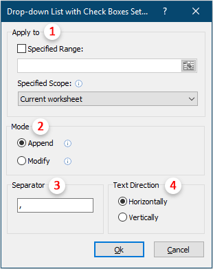
2. I Listruta med inställningar för kryssrutor dialogrutan, konfigurera så här.

  • 2.1) I Ansök till avsnittet, ange tillämpningsområdet där du skapar kryssrutor för objekt i listrutan. Du kan ange en visst intervall, nuvarande kalkylblad, aktuell arbetsbok or alla öppnade arbetsböcker baserat på dina behov.
  • 2.2) I Mode avsnitt, välj en stil som du vill mata ut de valda objekten;
  • Här tar Ändra alternativ som ett exempel, om du väljer detta kommer cellvärdet att ändras baserat på de valda objekten.
  • 2.3) I Separator rutan, ange en avgränsare som du kommer att använda för att separera flera objekt;
  • 2.4) I Textriktning avsnitt, välj en textriktning baserat på dina behov;
  • 2.5) Klicka på OK knapp.

3. Klicka på det sista steget Kutools > Listrutan > Listruta med kryssrutor > Aktivera rullgardinslista med kryssrutor för att aktivera den här funktionen.

Från och med nu, när du klickar på cellerna med rullgardinsmenyn i ett angivet omfång, kommer en listruta att dyka upp, välj objekt genom att markera kryssrutorna för att matas ut i cellen som nedanstående demo visas (Ta modifieringsläget som ett exempel ).

För mer information om den här funktionen, besök här.

  Om du vill ha en gratis provperiod (30 dagar) av det här verktyget, klicka för att ladda ner den, och gå sedan till för att tillämpa operationen enligt ovanstående steg.


Relaterade artiklar:

Autoslutför när du skriver i Excel-rullgardinsmenyn
Om du har en rullgardinsmeny för datavalidering med stora värden måste du bläddra nedåt i listan bara för att hitta rätt eller skriva hela ordet direkt i listrutan. Om det finns en metod för att automatiskt slutföra när du skriver den första bokstaven i rullgardinsmenyn blir allt enklare. Denna handledning ger metoden för att lösa problemet.

Skapa rullgardinslista från en annan arbetsbok i Excel
Det är ganska enkelt att skapa en rullgardinslista för datavalidering bland kalkylblad i en arbetsbok. Men om listdata du behöver för datavalideringen hittar du i en annan arbetsbok, vad skulle du göra? I den här guiden lär du dig hur du skapar en drop-down-lista från en annan arbetsbok i Excel i detalj.

Skapa en sökbar rullgardinslista i Excel
För en rullgardinsmeny med många värden är det inte lätt att hitta en riktig. Tidigare har vi introducerat en metod för automatisk komplettering av rullgardinsmenyn när du anger den första bokstaven i rullgardinsmenyn. Förutom funktionen för autoslutförande kan du också göra listrutan sökbar för att förbättra arbetseffektiviteten för att hitta rätt värden i listrutan. För att göra rullgardinsmenyn sökbar, prova metoden i den här självstudien.

Fyll i andra celler automatiskt när du väljer värden i Excel-listrutan
Låt oss säga att du har skapat en rullgardinslista baserat på värdena i cellområdet B8: B14. När du väljer något värde i listrutan vill du att motsvarande värden i cellintervall C8: C14 fylls automatiskt i en vald cell. För att lösa problemet kommer metoderna i denna handledning att göra dig en tjänst.

Fler handledning för rullgardinsmenyn ...

Bästa kontorsproduktivitetsverktyg

🤖 Kutools AI Aide: Revolutionera dataanalys baserat på: Intelligent utförande   |  Generera kod  |  Skapa anpassade formler  |  Analysera data och generera diagram  |  Anropa Kutools funktioner.
Populära funktioner: Hitta, markera eller identifiera dubbletter   |  Ta bort tomma rader   |  Kombinera kolumner eller celler utan att förlora data   |   Rund utan formel ...
Superuppslag: Flera kriterier VLookup    VLookup med flera värden  |   VSök över flera ark   |   Fuzzy Lookup ....
Avancerad rullgardinslista: Skapa snabbt en rullgardinslista   |  Beroende rullgardinslista   |  Flervals-rullgardinslista ....
Kolumnhanterare: Lägg till ett specifikt antal kolumner  |  Flytta kolumner  |  Växla synlighetsstatus för dolda kolumner  |  Jämför intervall och kolumner ...
Utvalda funktioner: Rutnätsfokus   |  Designvy   |   Stor formelbar    Arbetsbok & Bladhanterare   |  Resursbibliotek (Automatisk text)   |  Datumväljare   |  Kombinera arbetsblad   |  Kryptera/Dekryptera celler    Skicka e-postmeddelanden efter lista   |  Superfilter   |   Specialfilter (filtrera fet/kursiv/genomstruken...) ...
Topp 15 verktygssatser12 text verktyg (lägga till text, Ta bort tecken, ...)   |   50+ Diagram Typer (Gantt Chart, ...)   |   40+ Praktiskt Formler (Beräkna ålder baserat på födelsedag, ...)   |   19 Införande verktyg (Infoga QR-kod, Infoga bild från sökväg, ...)   |   12 Konvertering verktyg (Siffror till ord, Valutaväxling, ...)   |   7 Slå ihop och dela verktyg (Avancerade kombinera rader, Dela celler, ...)   |   ... och mer

Uppgradera dina Excel-färdigheter med Kutools för Excel och upplev effektivitet som aldrig förr. Kutools för Excel erbjuder över 300 avancerade funktioner för att öka produktiviteten och spara tid.  Klicka här för att få den funktion du behöver mest...

Beskrivning


Fliken Office ger ett flikgränssnitt till Office och gör ditt arbete mycket enklare

  • Aktivera flikredigering och läsning i Word, Excel, PowerPoint, Publisher, Access, Visio och Project.
  • Öppna och skapa flera dokument i nya flikar i samma fönster, snarare än i nya fönster.
  • Ökar din produktivitet med 50 % och minskar hundratals musklick för dig varje dag!
Comments (70)
No ratings yet. Be the first to rate!
This comment was minimized by the moderator on the site
Hello-

This is fabulous, but I was wondering if there is a way to call the code as a subroutine, ie Click Button 1, run this code with X List Box and X Output cell. I want to pass the listbox and the output cell as variables into this code. Any help would be greatly appreciated.

I've tried this:
Private Sub Rectangle1_Click()
Call MultiSelctDropdown(ListBox1,Output1)
End Sub

Private Sub Rectangle2_Click()
Call MultiSelctDropdown(ListBox2,Output2)
End Sub

Private Sub MultiSelectDropdown(ListBox As String, Output As String)
Dim xSelShp As Shape, xSelLst As Variant, I, J As Integer
Dim xV As String
Set xSelShp = ActiveSheet.Shapes(Application.Caller)
Set xLstBox = ActiveSheet.ListBox
If xLstBox.Visible = False Then
xLstBox.Visible = True
xSelShp.TextFrame2.TextRange.Characters.Text = "Enter"
xStr = ""
xStr = Range("Output").Value

If xStr <> "" Then
xArr = Split(xStr, ",")
For I = xLstBox.ListCount - 1 To 0 Step -1
xV = xLstBox.List(I)
For J = 0 To UBound(xArr)
If xArr(J) = xV Then
xLstBox.Selected(I) = True
Exit For
End If
Next
Next I
End If
Else
xLstBox.Visible = False
xSelShp.TextFrame2.TextRange.Characters.Text = "Click Here to Select Products"
For I = xLstBox.ListCount - 1 To 0 Step -1
If xLstBox.Selected(I) = True Then
xSelLst = xLstBox.List(I) & "," & xSelLst
End If
Next I
If xSelLst <> "" Then
Range("Output") = Mid(xSelLst, 1, Len(xSelLst) - 1)
Else
Range("Output") = ""
End If
End If
End Sub
This comment was minimized by the moderator on the site
Ok I figured this one out (see below)

But now I want to have only ONE list box that I can use over and over again with different buttons but different output depending on the button pushed. And the code below works for this EXCEPT the items selected when the list box pops up includes all items that have been outputted from the code.

If list box1 contains

Apples
Oranges
Pears
Kiwi

and button 1 is pressed and Apples is selected, when button 2 is pressed Apples is already selected, and if during button press 2 pears is selected when you go back to button 1 Apples AND Pears are selected.

How can I either clear all selected when a button is pressed OR make the selected options equal to the output.


Private Sub Button1_Click()
Call ProductSelection(ActiveSheet.ListBox1, "Button1Output", 243, 215)
End Sub
Private Sub Button2_Click()
Call ProductSelection(ActiveSheet.ListBox1, "Button2Output", 472, 215)
End Sub


Private Sub ProductSelection(xListBox As Object, Output As String, left As Integer, height As Integer)
Dim xSelShp As Shape, xSelLst As Variant, I, J As Integer
Dim xV As String
Set xSelShp = ActiveSheet.Shapes(Application.Caller)
Set xLstBox = xListBox
If xLstBox.Visible = False Then
xLstBox.Visible = True
xLstBox.left = left
xLstBox.height = height
xSelShp.TextFrame2.TextRange.Characters.Text = "Enter"
xStr = ""
xStr = Range(Output).Value

If xStr <> "" Then
xArr = Split(xStr, ",")
For I = xLstBox.ListCount - 1 To 0 Step -1
xV = xLstBox.List(I)
For J = 0 To UBound(xArr)
If xArr(J) = xV Then
xLstBox.Selected(I) = True
Exit For
End If
Next
Next I
End If
Else
xLstBox.Visible = False
xSelShp.TextFrame2.TextRange.Characters.Text = "Click Here to Select Products"
For I = xLstBox.ListCount - 1 To 0 Step -1
If xLstBox.Selected(I) = True Then
xSelLst = xLstBox.List(I) & "," & xSelLst
End If
Next I
If xSelLst <> "" Then
Range(Output) = Mid(xSelLst, 1, Len(xSelLst) - 1)
Else
Range(Output) = ""
End If
End If
End Sub
This comment was minimized by the moderator on the site
Hi there- this is super helpful, thank you! Can you tell me how I can draw a list box based on a list in a different worksheet (but same file)? I've tried entering my worksheet name (i.e., 'lists') followed by the range in the list fill range (after clicking on Properties) but this does not work.Thanks!
This comment was minimized by the moderator on the site
Hi Meghan,Supposing you want to <span style="letter-spacing: 0.2px; color: inherit; font-family: inherit; font-style: inherit; font-variant-ligatures: inherit; font-variant-caps: inherit;">ListBox1</span><span style="letter-spacing: 0.2px; color: inherit; font-family: inherit; font-style: inherit; font-variant-ligatures: inherit; font-variant-caps: inherit;">Sheet1</span><div data-tag="code">Sub listboxlistfillrangefromdifferentsheet()
Sheet1.ListBox1.ListFillRange = Sheet2.Range("A2:A20").Address(, , , True)
End Sub
This comment was minimized by the moderator on the site
hello, I have a problem with the list box: to make the list going down, I have to click on the box that allows the list to go down but when I click, it does not go down automatically, I have to click outside the list so that it refreshes and the list goes down, what to do? Thank you
This comment was minimized by the moderator on the site
Hi,You can't scroll ActiveX Listbox by mouse wheel. There is no setting for it.

This comment was minimized by the moderator on the site
Hi, thank you for sharing this! I have a question though, is it possible to populate different cells based on the selected option?For example, instead of having everything in one cell, each selection is populated in the cell below the earlier selection. Thank you!
This comment was minimized by the moderator on the site
Hi faez,
The VBA below helps to populate the selected options in different cells on the same row. Please have a try.

Sub Rectangle2_Click()
'Updated by Extendoffice 20211124
Dim xSelShp As Shape, xSelLst As Variant, I As Integer
Dim xRg As Range
Set xSelShp = ActiveSheet.Shapes(Application.Caller)
Set xLstBox = ActiveSheet.ListBox1
If xLstBox.Visible = False Then
xLstBox.Visible = True
xSelShp.TextFrame2.TextRange.Characters.Text = "Pickup Options"
Else
xLstBox.Visible = False
xSelShp.TextFrame2.TextRange.Characters.Text = "Select Options"
Set xRg = Range("ListBoxOutput")
For I = 0 To xLstBox.ListCount - 1
If xLstBox.Selected(I) = True Then
xSelLst = xLstBox.List(I)
xRg.Value = Mid(xSelLst, 1, Len(xSelLst))
Set xRg = xRg.Offset(0, 1)
End If
Next I
End If
End Sub
This comment was minimized by the moderator on the site
Hi Crystal,
Thanks a lot for this code, very helpful and convenient. One question : how to adpat it in order not to have the separator ";" if only one item is selected ?
This comment was minimized by the moderator on the site
Hi Eloi,No separator is displayed when you select only one item in the list.
This comment was minimized by the moderator on the site
Thanks Crystal, the mistake was in my adaptation of the code.
If someone needs to adapt it with a click on a cell instead of a click on a shape, you could try this (with a call to this sub in your sheet, with a condition when your cell is selected)

Sub affichage_liste(xLstBox As MSForms.ListBox, texte1 As String)
'Updated by Extendoffice 20200730
Dim xSelLst As Variant, I, J As Integer
Dim xV As String

If xLstBox.Visible = False Then
xLstBox.Visible = True
xStr = ""
xStr = Range(texte1).Value

If xStr <> "" Then
xArr = Split(xStr, ";")
For I = xLstBox.ListCount - 1 To 0 Step -1
xV = xLstBox.List(I)
For J = 0 To UBound(xArr)
If xArr(J) = xV Then
xLstBox.Selected(I) = True
Exit For
End If
Next
Next I
End If
Else
xLstBox.Visible = False
For I = xLstBox.ListCount - 1 To 0 Step -1
If xLstBox.Selected(I) = True Then
xSelLst = xLstBox.List(I) & "; " & xSelLst
End If
Next I
If xSelLst <> "" Then
Range(texte1) = Mid(xSelLst, 1, Len(xSelLst) - 2)
Else
Range(texte1) = ""
End If
End If
End Sub
This comment was minimized by the moderator on the site
Hi Eloi,The code you provided doesn't seem to work. I have modified it again as below.  After adding the code in your Sheet(Code) window, go back to the worksheet, click the cell C4 to expand the list box, after selecting items from the list box, click on any cell in the worksheet to output the selection, and no separator is displayed when you select only one item in the list.
<div data-tag="code">Private Sub Worksheet_SelectionChange(ByVal Target As Range)
'Updated by Extendoffice 20211223
Dim xSelLst As Variant, I, J As Integer
Dim xV As String
Set xLstBox = ActiveSheet.ListBox1

If Target.Address = "$C$4" Then


If xLstBox.Visible = False Then
xLstBox.Visible = True
xStr = ""
xStr = Range("ListBoxOutput").Value

If xStr <> "" Then
xArr = Split(xStr, ";")
For I = xLstBox.ListCount - 1 To 0 Step -1
xV = xLstBox.List(I)
For J = 0 To UBound(xArr)
If xArr(J) = xV Then
xLstBox.Selected(I) = True
Exit For
End If
Next
Next I
End If

End If

Else
xLstBox.Visible = False

For I = xLstBox.ListCount - 1 To 0 Step -1
If xLstBox.Selected(I) = True Then
xSelLst = xLstBox.List(I) & "; " & xSelLst
End If
Next I
If xSelLst <> "" Then
Range("ListBoxOutput") = Mid(xSelLst, 1, Len(xSelLst) - 2)
Else
Range("ListBoxOutput") = ""
End If


End If

End Sub
This comment was minimized by the moderator on the site
Thanks a lot Crystal
This comment was minimized by the moderator on the site
Bonjour,Je suis plus que novice sur excel étant sur mac je ne peux utiliser l'outil Kutools j'ai donc tenté de créer une liste déroulante où l'on peut cocher plusieurs items mais je bloque dès le début dans l'onglet développeur puisque je n'ai pas du tout l'outil "insert".Merci pour votre aide
This comment was minimized by the moderator on the site
Hi I am newbie to VBA. I tried to execute the code but i get the following error "Run-time error '-2147024809 (80070057)': The Item with the specified name wasn't found". Can you help me with this
This comment was minimized by the moderator on the site
Hi Gowtham,It seem that this error occurs when you running the code directly in the Code editor (the Microsoft Visual Basic for Applications window).After adding the code, please press the Alt + Q keys to close the Microsoft Visual Basic for Applications window. Go back to the worksheet and execute the code by clicking the rectangle button (see the .gif picture in step 6).
This comment was minimized by the moderator on the site
Hi Crystal, even after your tip am getting same error as Gowtham. My error is right after protect my sheet. Would you please help me with this issue?
This comment was minimized by the moderator on the site
Hi Crystal, Even After your tip I am getting same error as Gowtham.
This comment was minimized by the moderator on the site
Hi Mina,Which Excel and Windows version are you using?
This comment was minimized by the moderator on the site
Hello,I added this code to an existing macro template and it is loading the selections correctly, but it is NOT clearing out the x on the selected items..This will be used on/in a template worksheet that has submit button/macro to load the worksheet answers into a hidden worksheet with a data table.And am happy to say the field data loaded to the cell, transferred into my variable, and loaded to the data table as expected.
This code was a HUGE blessing!
I use excel 2016
How do I fix this. I am using this version from below.
Sub Rectangle1_Click()
'Updated by Extendoffice 20200730
Dim xSelShp As Shape, xSelLst As Variant, I, J As Integer
Dim xV As String
Set xSelShp = ActiveSheet.Shapes(Application.Caller)
Set xLstBox = ActiveSheet.ListBox1
If xLstBox.Visible = False Then
xLstBox.Visible = True
xSelShp.TextFrame2.TextRange.Characters.Text = "Pickup Options"
xStr = ""
xStr = Range("ListBoxOutput").Value

If xStr <> "" Then
xArr = Split(xStr, ";")
For I = xLstBox.ListCount - 1 To 0 Step -1
xV = xLstBox.List(I)
For J = 0 To UBound(xArr)
If xArr(J) = xV Then
xLstBox.Selected(I) = True
Exit For
End If
Next
Next I
End If
Else
xLstBox.Visible = False
xSelShp.TextFrame2.TextRange.Characters.Text = "Select Options"
For I = xLstBox.ListCount - 1 To 0 Step -1
If xLstBox.Selected(I) = True Then
xSelLst = xLstBox.List(I) & ";" & xSelLst
End If
Next I
If xSelLst <> "" Then
Range("ListBoxOutput") = Mid(xSelLst, 1, Len(xSelLst) - 1)
Else
Range("ListBoxOutput") = ""
End If
End If
End Sub
This comment was minimized by the moderator on the site
Hello,

I'm having a similar problem to Tom from 2 months ago. When I try to share my file with a colleague, the multi-select droplist list isn't working. However, I used the Kutools add-on to create this as opposed to creating it myself. I've also saved it as macro-enabled.
This comment was minimized by the moderator on the site
Hi ben,The multi-select drop down list feature of Kutools only works in the Excel that installed our Kutools. We are working on this issue, sorry for the inconvenience.
This comment was minimized by the moderator on the site
Hello I looking the resolve for problem with saving choosing on drop down list

when i choose something on list and send file to my colleague, then when he open file and want to check my list then list has cleared and cell "ListBoxOutput" was cleared too.

help please :)
This comment was minimized by the moderator on the site
Hi Tom,
Please save the workbook as an "Excel MacroEnable Workbook" and then send this .xlsm file to your colleague.
This comment was minimized by the moderator on the site
hello i save this file in this format from beginning ;), but without effect. still when i fill file and send to someone then when he opened file and click to "shape" then macro started from begin and cleared list
This comment was minimized by the moderator on the site
Hi Tom,
I am sorry for the mistake. The code has been updated again. Please have a try.

Sub Rectangle1_Click()

'Updated by Extendoffice 20200730

Dim xSelShp As Shape, xSelLst As Variant, I, J As Integer

Dim xV As String

Set xSelShp = ActiveSheet.Shapes(Application.Caller)

Set xLstBox = ActiveSheet.ListBox1

If xLstBox.Visible = False Then

xLstBox.Visible = True

xSelShp.TextFrame2.TextRange.Characters.Text = "Pickup Options"

xStr = ""

xStr = Range("ListBoxOutput").Value


If xStr <> "" Then

xArr = Split(xStr, ";")

For I = xLstBox.ListCount - 1 To 0 Step -1

xV = xLstBox.List(I)

For J = 0 To UBound(xArr)

If xArr(J) = xV Then

xLstBox.Selected(I) = True

Exit For

End If

Next

Next I

End If

Else

xLstBox.Visible = False

xSelShp.TextFrame2.TextRange.Characters.Text = "Select Options"

For I = xLstBox.ListCount - 1 To 0 Step -1

If xLstBox.Selected(I) = True Then

xSelLst = xLstBox.List(I) & ";" & xSelLst

End If

Next I

If xSelLst <> "" Then

Range("ListBoxOutput") = Mid(xSelLst, 1, Len(xSelLst) - 1)

Else

Range("ListBoxOutput") = ""

End If

End If

End Sub
This comment was minimized by the moderator on the site
Now it's working perfectly.

Many thanks for your help
There are no comments posted here yet
Load More
Please leave your comments in English
Posting as Guest
×
Rate this post:
0   Characters
Suggested Locations